Automated Content Analysis with R
Topic modeling
Cornelius Puschmann & Mario Haim
Compared to the dictionary approach, topic modeling is a much more recent and demanding procedure when it comes to the computing power and memory requirements of your computer. Topic models are mathematically complex and completely inductive (i.e., the model does not require any knowledge of the content, but this does not mean that such knowledge is not crucial for validating the output). The relationship of topics to words and documents is fully automated in a topic model. The best-known implementation today is the so-called Latent Dirichlet Allocation (or LDA for short) and was developed by the computer linguists David Blei, Andrew Ng, and Michael Jordan (the other one). In contrast to previous chapters, topic modeling requires a more in-depth understanding of the underlying algorithms – it is however sufficient to try them out and (and this is very important!) systematically check the quality of the results obtained (i.e., validate the model comprehensively). This is done by means of a series of procedures which evaluate the fit of the model in relation to variables such as the number of topics selected. While the preceding approaches often produce results that need to be carefully checked, topic-model results are particularly difficult to predict because the inductive word distribution patterns on which topic models are based, sometimes differ greatly from the human understanding of a topic.
Since topic models are not part of quanteda’s equipment, we use two new packages for their calculation: topicmodels and stm. The topicmodels package implements the two methods Latent Dirichlet Allocation (LDA) and Correlated Topic Models (CTM), while STM is based on a completely new approach, which contains numerous extensions compared to LDA. Besides these packages, we will also be using the libraries ldatuning and wordcloud to optimize and plot models.
if(!require("quanteda")) {install.packages("quanteda"); library("quanteda")}
if(!require("tidyverse")) {install.packages("tidyverse"); library("tidyverse")}
if(!require("topicmodels")) {install.packages("topicmodels"); library("topicmodels")}
if(!require("ldatuning")) {install.packages("ldatuning"); library("ldatuning")}
if(!require("stm")) {install.packages("stm"); library("stm")}
if(!require("wordcloud")) {install.packages("wordcloud"); library("wordcloud")}
theme_set(theme_bw())
LDA topic modeling with the Sherlock corpus
We start with a very simple LDA topic model, which we calculate using the topicmodels package. This package offers hardly any functions to inspect the model, but a look at the object structure helps, if you are at least roughly familiar with topic models. At the end of this section, we’ll discuss how to extract the most important metrics from an LDA model.
First, we load the Sherlock-Holmes corpus again, but this time in a special variant. The version used below divides the corpus into 174 documents, each consisting of 40 sentences. We have already performed this step using the corpus_reshape function. The result is 10-17 “texts” per novel, as if the novels were divided into chapters, which they are not in the version we use.
Why this effort? For the LDA analysis, the number of only 12 (relatively long) texts is altogether less favourable than this division, even if the arbitrary division according to the number of sentences works less well than the meaningful capitals would do. Here is an overview of the refactored corpus.
load("data/sherlock/sherlock.absaetze.RData")
as.data.frame(korpus.stats)
Second, and already well-known, we calculate a DFM and remove numbers, symbols and English standard stop words. Also, we remove those terms that occur only once, as well as those that occur more than 75 times. The command dfm_trim allows more complex parameters like the term frequency relative to the term frequency or the document frequency as a whole, but at this point this simple filtering is sufficient.
sherlock.dfm <- dfm(korpus, remove_numbers = TRUE, remove_punct = TRUE, remove_symbols = TRUE, remove = c(stopwords("english"), "sherlock", "holmes"))
dfm.trim <- dfm_trim(sherlock.dfm, min_termfreq = 2, max_termfreq = 75)
dfm.trim
## Document-feature matrix of: 174 documents, 4,226 features (96.3% sparse).Third, we not turn to the actual modeling of the topics. That is, we arbitrarily define a number of topics of k = 10. The number of topics is basically variable and is determined on the basis of different factors (it is also both very crucial and controversial; but more on that later). Then we convert the quanteda DFM with the already known command convert into a format which is also digestable by the package topicmodels. While the previously used commands came from quanteda, the LDA command is now taken from the topicmodels package.
n.topics <- 10
dfm2topicmodels <- convert(dfm.trim, to = "topicmodels")
lda.model <- LDA(dfm2topicmodels, n.topics)
lda.model
## A LDA_VEM topic model with 10 topics.Fourth and after the actual model has been calculated, we can now output two central components of the model: The terms that are particularly strongly linked to each of the topics (with the command terms) …
as.data.frame(terms(lda.model, 10))… and the documents in which the topics are particularly strong (with the command topics).
data.frame(Topic = topics(lda.model))What exactly do we see here? The first table shows the ten most closely related terms for each of the ten topics. The second table again shows the topic with the highest proportion for each text. As already explained, “texts” in this case are actually paragraphs from individual novels, so “01_02” is the second paragraph of A Scandal in Bohemia.
For terms and texts alike, all topics are linked to all terms/texts in a certain strength. Yet, we are usually only interested in associations of a certain strength.
What quantitative distribution results from this? This can be easily determined by dividing the thematic events for a novel by the total number of sections.
lda.topics.chapters <- data.frame(korpus.stats, Topic = topics(lda.model)) %>%
  add_count(Roman, Topic) %>%
  group_by(Roman) %>%
  mutate(Share = n/sum(n)) %>%
  ungroup() %>%
  mutate(Topic = paste0("Topic ", sprintf("%02d", Topic))) %>%
  mutate(Novel = as_factor(Roman))
ggplot(lda.topics.chapters, aes(Novel, Share, color = Topic, fill = Topic)) + geom_bar(stat="identity") + ggtitle("LDA topics in Sherlock Holmes novels") + xlab("") + ylab("Share of topics [%]") + theme(axis.text.x = element_text(angle = 45, hjust = 1))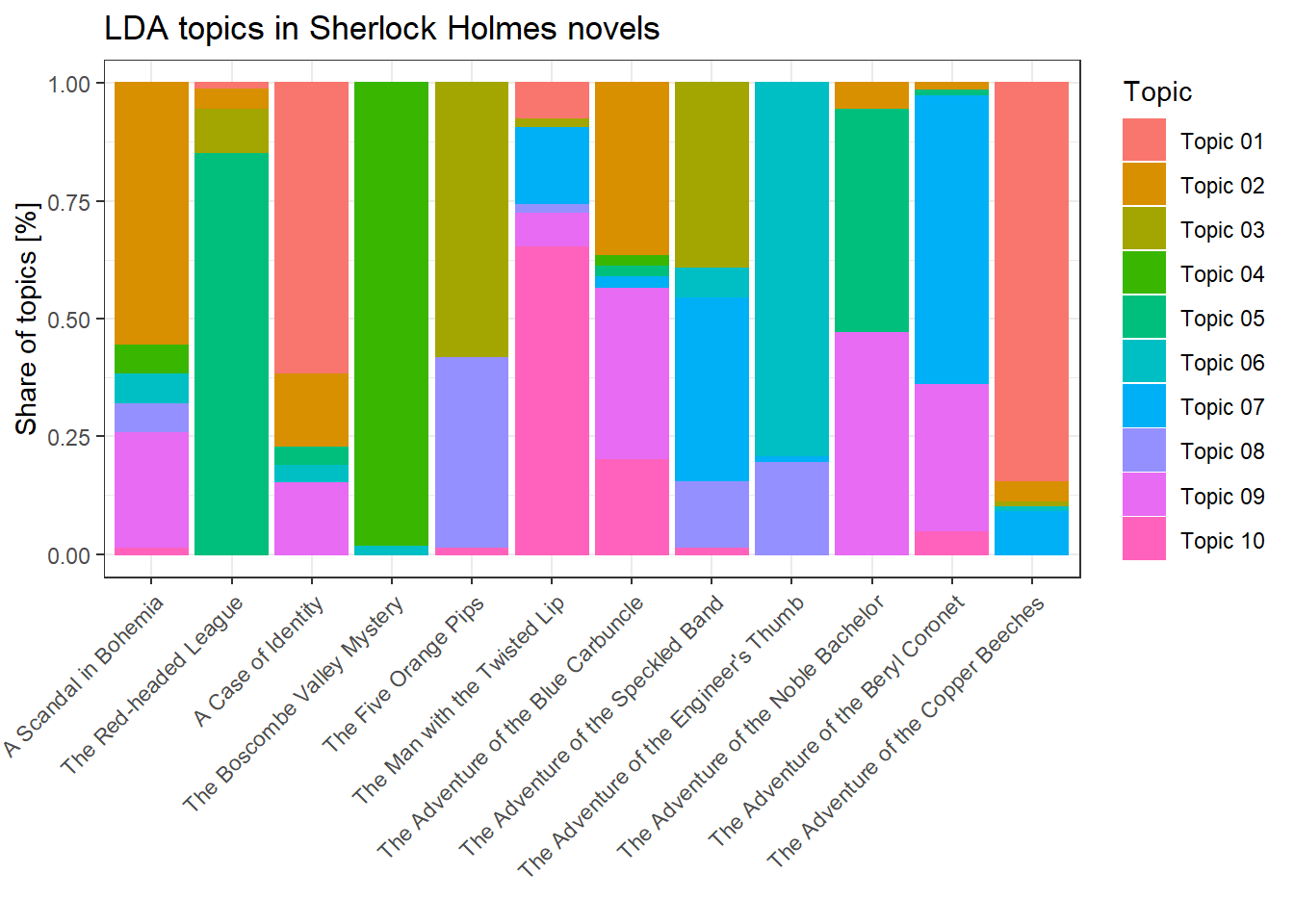
It is immediately obvious that several novels have their own theme, which is quite understandable given the characteristics of the novel genre. However, there are also topics that appear in several novels and are more general in nature, or that include characters that appear in a variety of Sherlock-Holmes narratives.
In this example, the distribution of themes in documents is calculated somewhat differently than usual, because we perform this step manually, so to speak, using functions from dplyr. The “normal” calculation of the relationship between terms and topics or documents and topics is done by extracting the variables beta and gamma that are already contained in the LDA model (the structure of the model can be examined more closely with the standard R command str). The result is a data frame, which can of course also be plotted. The variables V1-VX denote the topics here, while the lines contain the terms or the documents. The number values describe the probability of the association of a term with a topic, or the share of a topic in a document.
head(as.data.frame(t(lda.model@beta), row.names = lda.model@terms)) # Terms > Topicshead(as.data.frame(lda.model@gamma, row.names = lda.model@documents)) # Documents > TopicsWhat did we learn from the model? First of all, there are topics that essentially reflect the plot of the novel in question. This is not surprising given the comparatively small sample – a much larger corpus would give us better results. On the other hand, however, there are also recognizable topics that are not bound to a single novel, but occur in several novels. Nevertheless, the genre – novels of the same author on the (roughly) same topic – is not ideal for a sound analysis with LDA.
LDA topic (count) tuning
Before we turn to this example, let’s take a look at a heuristic for determining the ideal k (i.e., the a-priori specified number of topics). Instead of simply specifying an arbitratry number, it makes sense to test the fit of different settings. This is facilitated by the LDAtuning package, which includes a number of different metrics for determining a good number of topics based on statistical factors. Attention: this calculation is very time-consuming because a separate model is calculated for each step (15 individual models in this example). This can easily take several days, especially for larger data sets.
ldatuning.metrics <- FindTopicsNumber(dfm2topicmodels, topics = seq(from = 2, to = 15, by = 1), metrics = c("Griffiths2004", "CaoJuan2009", "Arun2010", "Deveaud2014"), method = "Gibbs", control = list(seed = 77), mc.cores = 2L, verbose = TRUE
)
## fit models... done.
## calculate metrics:
## Griffiths2004... done.
## CaoJuan2009... done.
## Arun2010... done.
## Deveaud2014... done.Of course, also these tuned metrics can be plotted.
FindTopicsNumber_plot(ldatuning.metrics)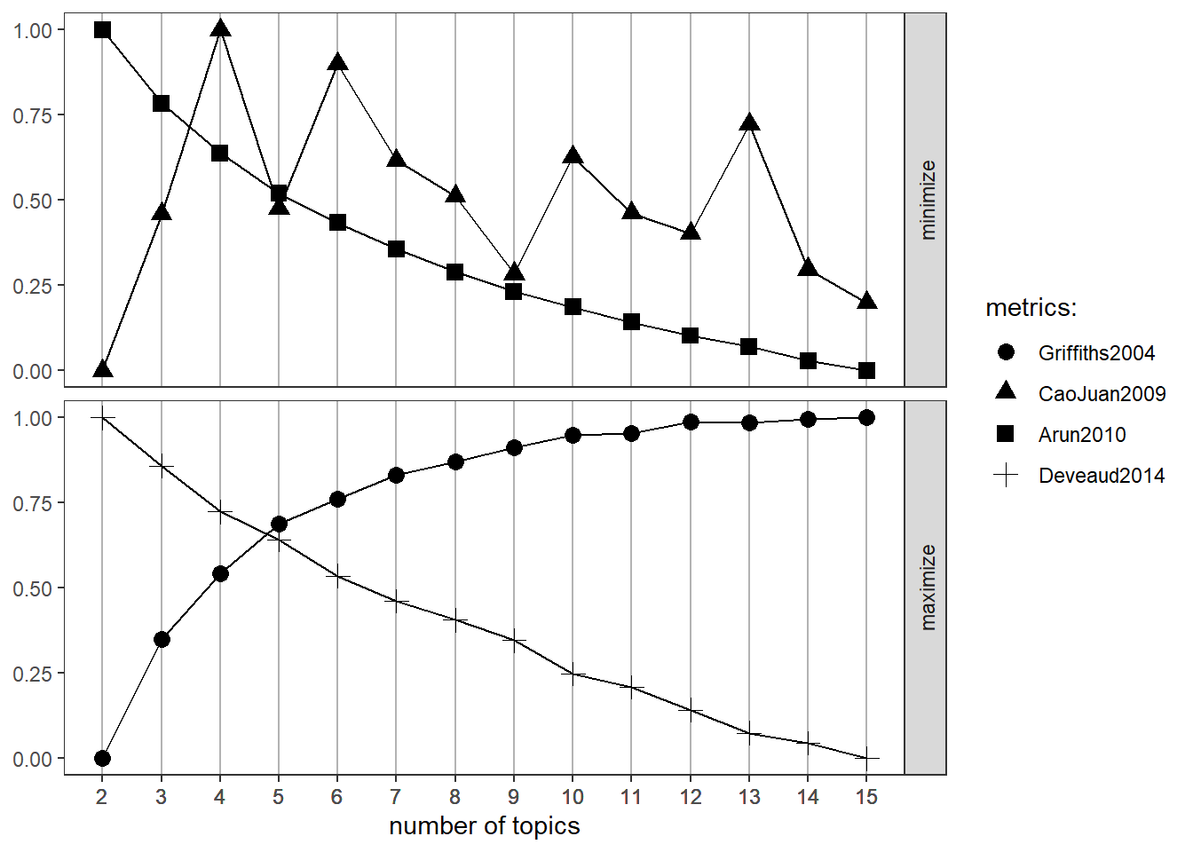
The results are somewhat inconsistent, which, again, is primarily due to the fact that the data do not represent an ideal basis for a topic model using LDA. Two metrics (Arun et al, 2010 and Griffiths & Steyvers, 2004) consistently improve and probably have their ideal point at k > 15, while the other two (Cao et al, 2009 and Deveaud, San Juan & Bellot, 2014) fluctuate and drop respectively.
STM topic modeling with the UN corpus
Now we turn to a topic-modeling approach that has been developed specifically for social-science applications and thus offers numerous additional functions compared to LDA: Structured Topic Models or STM. A very good introduction to STM is provided by this article by Molly Roberts and colleagues. The code used here strongly follows the examples from the article, even if we use different data.
Again, we first use quanteda and then “hand over” a DFM to the stm package that calculates the actual model. Again, we use the UN General Debate Corpus from previous chapters. First we load the prepared UN corpus data again.
load("data/un/un.korpus.RData")
head(korpus.un.stats, 100)
Then we calculate – you guessed it – a DFM excluding numbers, punctuation, symbols, and stop words, and reduce them again, in this case especially generously, by removing words that occur in less than 7.5% and more than 90% of all documents. This has to do with the size of the corpus, which allows us to strongly distill the content without losing really relevant information. Especially in this case, the calculation of the model becomes extremely slow if we do not effectively reduce the data, leaving behind “noise” which makes the analysis much more difficult.
dfm.un <- dfm(korpus.un, remove_numbers = TRUE, remove_punct = TRUE, remove_symbols = TRUE, remove = stopwords("english"))
dfm.un.trim <- dfm_trim(dfm.un, min_docfreq = 0.075, max_docfreq = 0.90, docfreq_type = "prop") # min 7.5% / max 90%
dfm.un.trim
## Document-feature matrix of: 7,897 documents, 2,479 features (77.3% sparse).Now we can calculate the STM model, which is initially similar to the LDA topic model. We define a number of topics of k = 40 and then convert the DFM from quanteda to a form that can be understood yy the stm package using convert.
Since the calculation of an STM model with a larger number of topics for an extensive corpus such as the UN General Debate Corpus takes much longer than in the previous examples, we load an already calculated model with load() in the following code block. If you want to look at the STM calculation in action, you only have to comment out the line with the function call of stm (i.e., remove the “#”).
Finally we create a table which shows us the most important keywords for each topic (X1-X40).
n.topics <- 40
dfm2stm <- convert(dfm.un.trim, to = "stm")
#modell.stm <- stm(dfm2stm$documents, dfm2stm$vocab, K = n.topics, data = dfm2stm$meta, init.type = "Spectral")
load("data/un/un.stm.RData")
as.data.frame(t(labelTopics(modell.stm, n = 10)$prob))
To look at the topics visually, we can rely on the package wordcloud and plot the STM topics as, well, a word cloud.
par(mar=c(0.5, 0.5, 0.5, 0.5))
cloud(modell.stm, topic = 1, scale = c(2.25,.5))
cloud(modell.stm, topic = 3, scale = c(2.25,.5))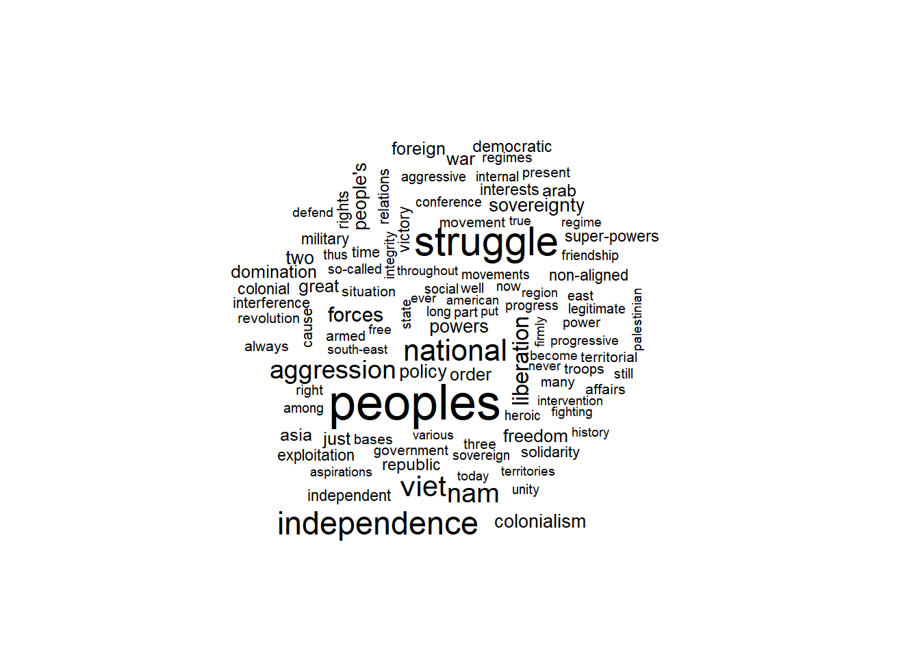
cloud(modell.stm, topic = 7, scale = c(2.25,.5))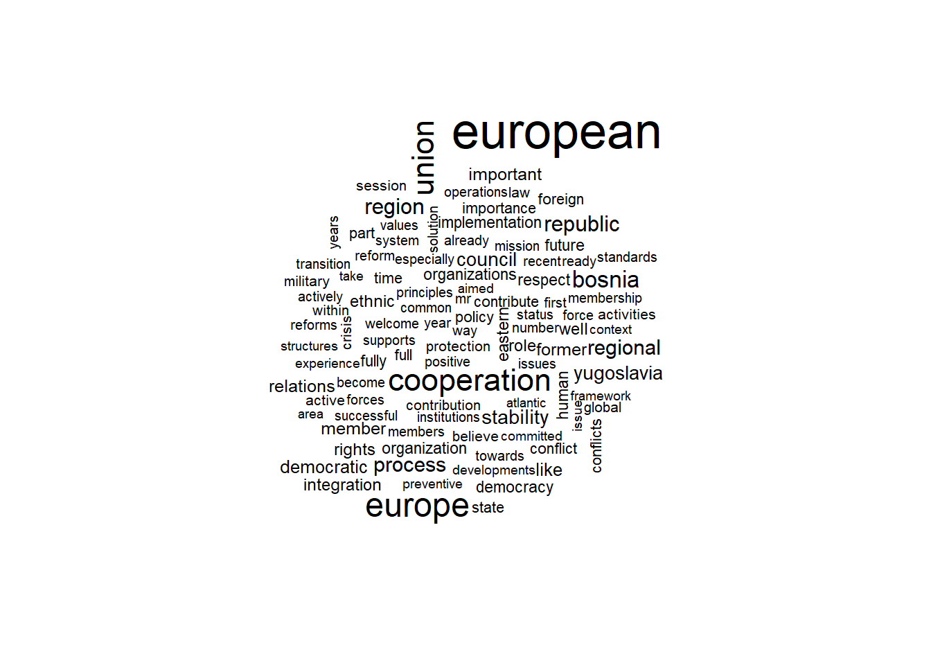
cloud(modell.stm, topic = 9, scale = c(2.25,.5))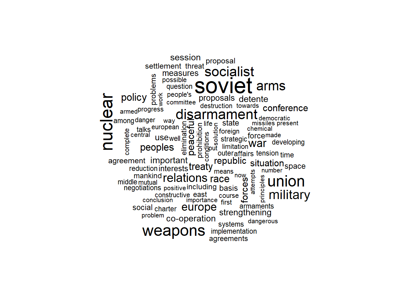
One practical aspect of STM models is that the plot.STM command, similar to quanteda, already integrates other plot types of its own into the package, which can display certain parts of the model (on topics, terms, documents) without having to convert this yourself.
The following four plots show (a) the respective Topic shares on the corpus as a whole, (b) a histogram of the topic shares within the documents, (c) central terms to four related topics, and (d) the contrasts between two related topics.
plot(modell.stm, type = "summary", text.cex = 0.5, main = "Topic shares on the corpus as a whole", xlab = "estimated share of topics")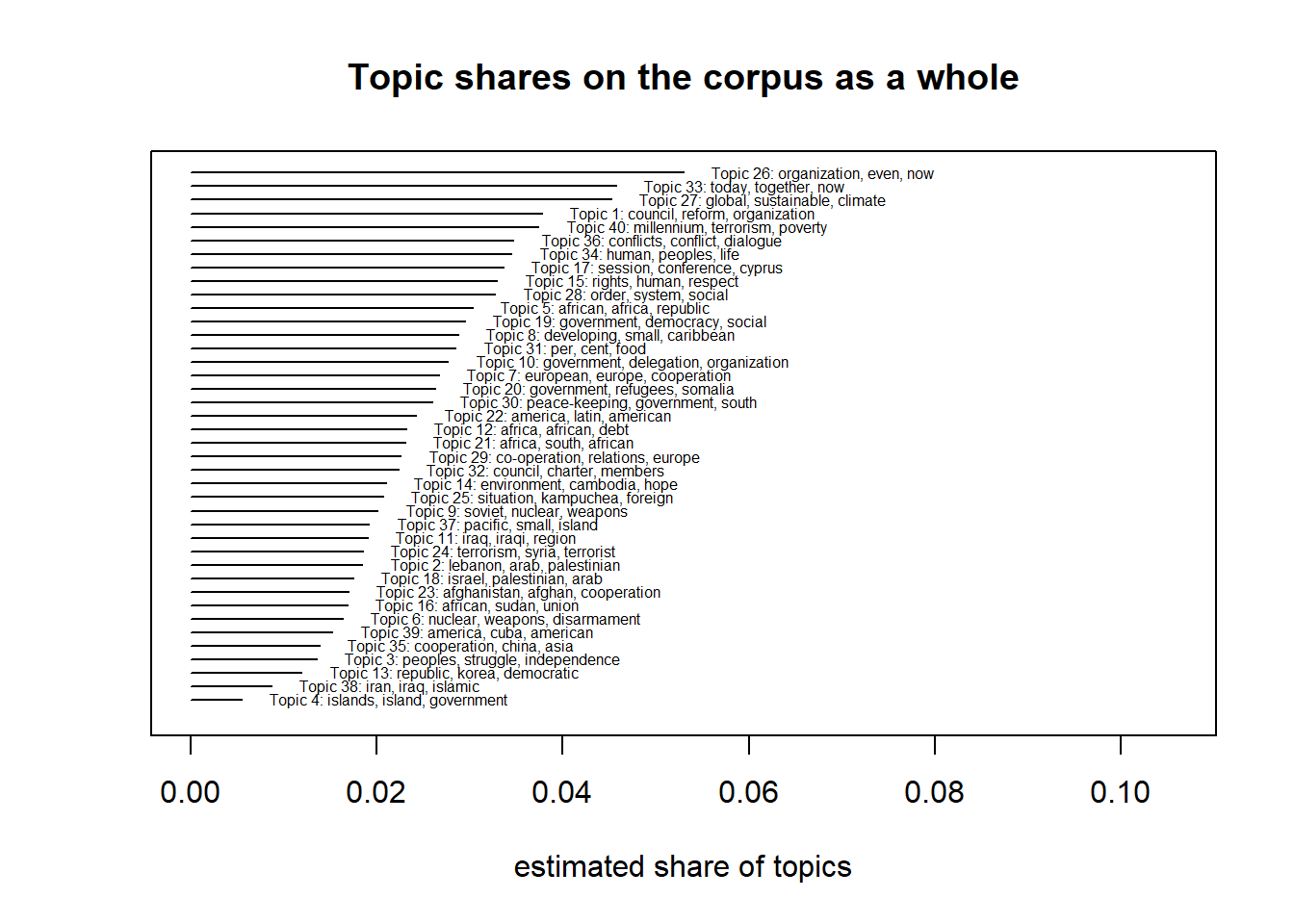
plot(modell.stm, type = "hist", topics = sample(1:n.topics, size = 9), main = "histogram of the topic shares within the documents")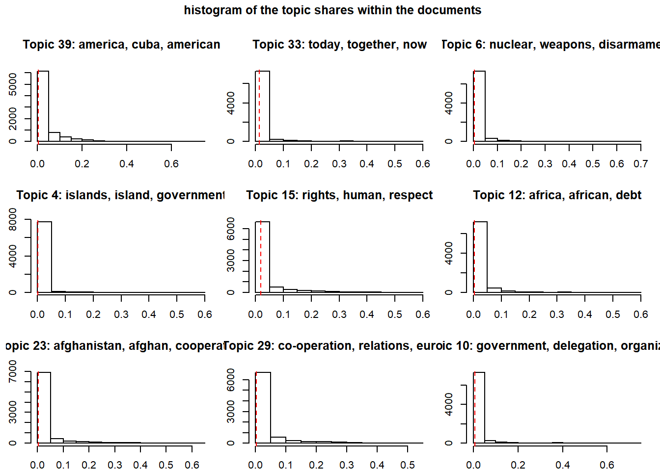
plot(modell.stm, type = "labels", topics = c(5, 12, 16, 21), main = "Topic terms")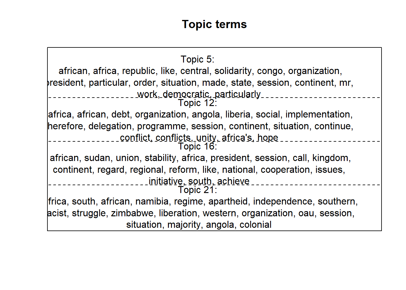
plot(modell.stm, type = "perspectives", topics = c(16,21), main = "Topic contrasts")
Next, we calculate the prevalence of the topics over time. For this we use the function estimateEffect, which is also part of stm and calculates a regression of the estimated topic parts. In contrast to LDA, where we also were able to determine topic shares (and thus a calculation of the shares by time would not have been an obstacle), estimateEffect can also take covariates into account, which can considerably increase the accuracy of the model. In addition, we get a local confidence interval for our estimate.
modell.stm.labels <- labelTopics(modell.stm, 1:n.topics)
dfm2stm$meta$datum <- as.numeric(dfm2stm$meta$year)
modell.stm.effekt <- estimateEffect(1:n.topics ~ country + s(year), modell.stm, meta = dfm2stm$meta)
We now plot the topic prevalence for nine selected topics. For better clarity, the most important key terms have been chosen as labels; the somewhat weird and unhandy loop structure becomes necessary in order to be able to compare a large number of topics directly.
par(mfrow=c(3,3))
for (i in 1:9)
{
  plot(modell.stm.effekt, "year", method = "continuous", topics = i, main = paste0(modell.stm.labels$prob[i,1:3], collapse = ", "), ylab = "", printlegend = F)
}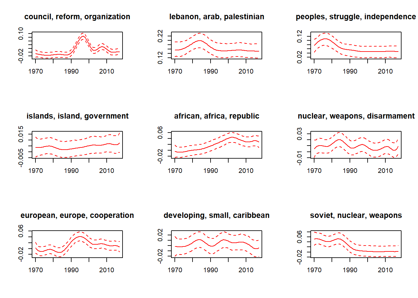
The results give reason to assume that interesting trends can actually be identified with STM topic models. First, the results are partly confirmatory: We would expect that a topic on Soviet nuclear weapons (here topic #9) would fall sharply with the end of the Soviet Union. The fact that the topic does not disappear completely has to do on the one hand with the fact that it continues to be mentioned, but also with the fact that it has contact with other topics (such as new Russian nuclear weapons). No topic model can make such differentiations perfectly, because some topics simply resemble each other too much, even if a person would recognize the difference without problems. We also note that certain topicss (in the sense of the model) contain individual historical events, sometimes in combination, such as the Lebanon War and the First Intifada (topic #2), the Second Congo War (topic #5), or the gradual realization of the European Monetary Union (topic #7). Other themes are less “timely” in comparison, with some hardly changing their level over time (Pacific island states, topic #4) and others recurring seasonally (nuclear disarmament, topic #6). Interesting is the sharp decrease on national (socialist) independence movements, which still played a visible role in the 1970s (topic #3), or discourses on UN and UN Security Council reform (topic #1).
How can the differences in the displayed confidence intervals be interpreted, we hear you ask? Well, topics such as the reform of the UN Security Council or the European cooperation can be identified more clearly in lexical terms than the (presumably quite variable) discourses on the interests of island states. Topics with a very clear temporal profile are generally more reliably identifiable than those that occur over longer periods of time.
STM topic (count) tuning
The (statistically) ideal number of topics can also be determined for an STM model. First we load the uninformative (but small) Sherlock Holmes dataset again. In the following code section, this is converted into a DFM and then converted (these steps are identical to those at the beginning of the chapter).
load("data/sherlock/sherlock.absaetze.RData")
sherlock.dfm <- dfm(korpus, remove_numbers = TRUE, remove_punct = TRUE, remove_symbols = TRUE, remove = c(stopwords("english"), "sherlock", "holmes"))
sherlock.dfm.trim <- dfm_trim(sherlock.dfm, min_termfreq = 2, max_termfreq = 75)
dfm2stm <- convert(sherlock.dfm.trim, to = "stm")
Now we use the function searchK, which comes directly from stm, just like we would use LDAtuning. This function also tries different k’s one after the other (i.e., you will need some time with you to use it, especially if you have a larger corpus than the one used in the example). Similar to the calculation above, in order to save time, we have already saved the result as an RData file, which can be plotted immediately. The functionality is the same as for the methods used in LDAtuning, the maximization or minimization of the characteristic values with increasing k. Here, too, the statistical methods do not provide any direct information as to how plausible the topics are necessarily for human readers.
load("data/sherlock/sherlock.stm.idealK.RData")
#mein.stm.idealK <- searchK(dfm2stm$documents, dfm2stm$vocab, K = seq(4, 20, by = 2), max.em.its = 75)
plot(mein.stm.idealK)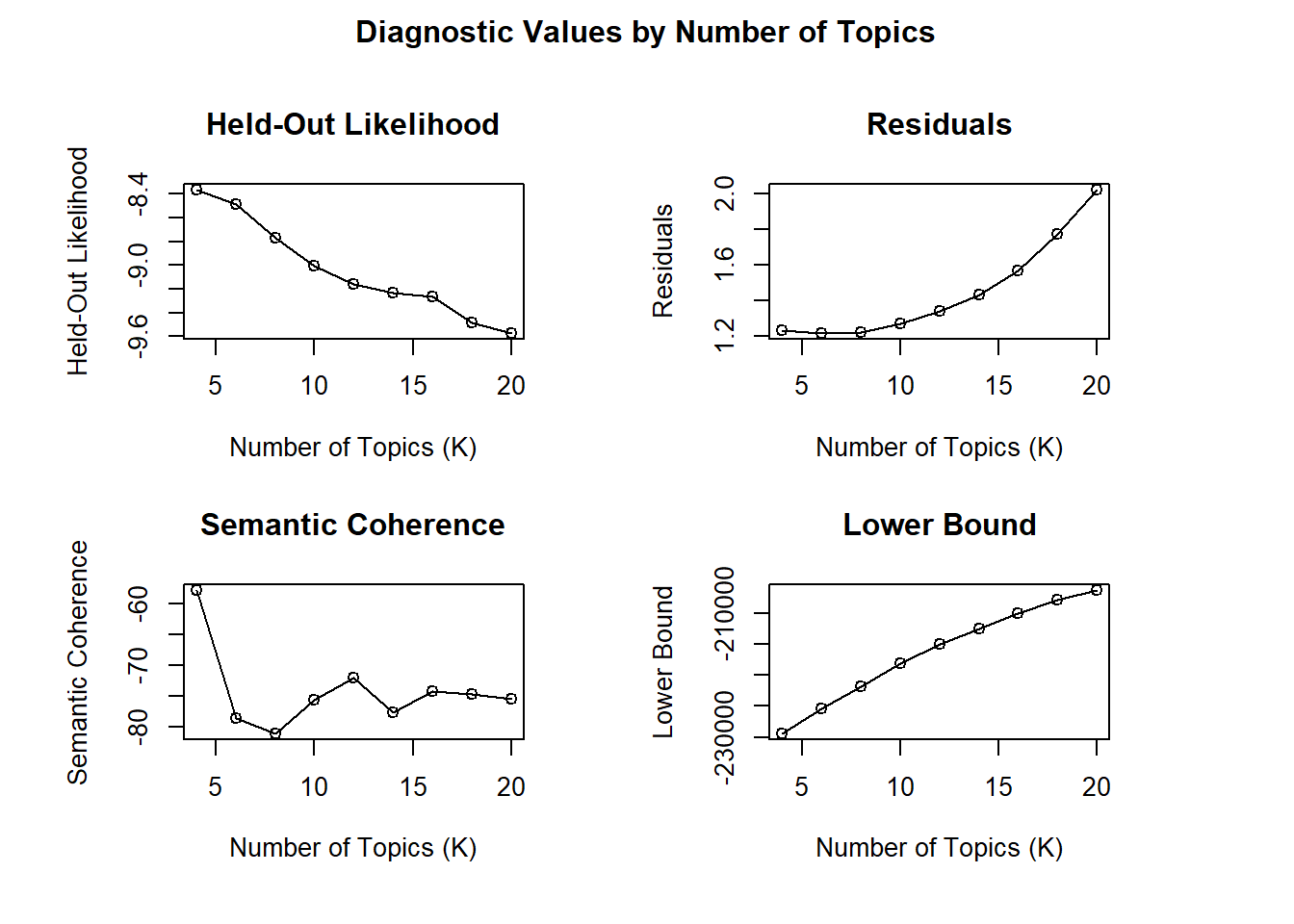
Things to remember about topic models
The following characteristics of topic models are worth bearing in mind:
- topic models are a useful tool for automated content analysis, both when exploring a large amount of data and when it comes to systematically identifying relationships between topics and other variables
- certain prerequisites such as minimum size and variety of the corpus (namely on the level of words and documents and their relation to each other) need to be met for a conclusive model
- everything above a certain degree of word frequencies is considered a “topic,” even if it is not a topic in human interpretation
- again, validate, validate, validate