Automated Content Analysis with R
Basics
Cornelius Puschmann & Mario Haim
The aim of this first chapter is to provide an introduction to quanteda, which we will use extensively in this course to analyze (textual) social-media content. In doing so, we will also cover basic concepts relevant in quantitative content analysis. In addition to quanteda, several other R libraries are used in this class, such as for supervised machine learning. The packages of the tidyverse (especially ggplot, dplyr, and stringr) are also relevant in practically every unit, as they greatly improve plotting, word processing, and data management over the basic R functions.
The basis of the analysis in this first section are the popular stories of Sherlock Holmes. The Sherlock Holmes corpus consists of twelve novels which are summarized in the volume The Adventures of Sherlock Holmes published in 1892 and which can be downloaded under the public domain from the Internet Archive. The version used for this introduction was first taken from the Internet Archive and then divided into twelve individual files. Of course, the methods presented here will later be applied to social-media data – the example only serves to slowly get used to quanteda and the basics of computer-aided content analysis.
Installing/loading R libraries
First, the necessary libraries are installed (if not already available) and then loaded. In addition, the theme setting for the package ggplot is set in preparation (this makes for nicer plots). We will repeat this step at the beginning of each chapter. In some sections, additional packages will be used, for example for an extended color palette (RColorBrewer), word clouds (wordcloud), or to parse URLs (urltools).
if(!require("quanteda")) {install.packages("quanteda"); library("quanteda")}
if(!require("readtext")) {install.packages("readtext"); library("readtext")}
if(!require("tidyverse")) {install.packages("tidyverse"); library("tidyverse")}
if(!require("RColorBrewer")) {install.packages("RColorBrewer"); library("RColorBrewer")}
theme_set(theme_bw())
Reading data
After all the necessary packages have been loaded, we can now import the Sherlock Holmes novels into a quanteda corpus. The readtext function from the package of the same name is used to import plaintext files, which can be used to successfully import a number of file formats (including TXT, PDF, and Word). Basically plaintext data (usually ending in “.txt”) and data in table form (e.g. in CSV format or as an Excel file) can be read by readtext without any major problems, but when importing, you have to specify how the individual data records are separated from each other (for plaintext files, for example, where not 1 file equals 1 text, which can be the case for exports from Lexis Nexis) and which fields contain the primary and meta data (for tables). A good introduction to the readtext package can be found here.
In this case, each file corresponds to one text, which makes the import very easy. We remove the “.txt” extension from the document name so that it can be used later in plot labels. We then create a corpus, which is the essential step to proceed further. Finally, the variable corpus is called, which returns the important key varialbe document number along other so-called “docvars” (metadata for the texts in the corpus).
sherlock <- readtext("data/sherlock/novels/[0-9]*.txt")
sherlock$doc_id <- str_sub(sherlock$doc_id, start = 4, end = -5)
my.corpus <- corpus(sherlock)
docvars(my.corpus, "Textno") <- sprintf("%02d", 1:ndoc(my.corpus))
my.corpus
## Corpus consisting of 12 documents and 1 docvar.Similarly, most analyses with quanteda consist of these three steps:
- Import raw textual data (from files or an API)
- Build a corpus (text + metadata)
- Calculate a document feature matrix (DFM)
Along the way we will also explore a few features that are helpful for cleaning, filtering, and pre-processing corpus data.
Now that we have read in the data stored in 12 files (one per novel) and generated a metadata variable that stores the index number of the respective text, we can continue to whatever analyses we fancy. Like, now, we will proceed to generating some corpus statistics.
Importantly, in the following chapters, we sometimes build on already prepared corpora. That is, instead of importing raw TXT files and generating the corpus format, we tend to directly import the corpus. This is to save computational ressources and hard-disk space.
Generating corpus statistics
After having imported the data and created a corpus, we now generate a set of basic corpus statistics. The ndoc, ntoken, ntype, and nsentence functions output the number of documents, tokens (the number of words), types (the number of unique words), and sentences in a corpus. These statistics can also be conveniently created along with document-level metadata using the summary function. While we now create an own variable for these statistics, for most corpora used in our examples, such a data frame with statistics for each text is already included. However, this is not necessary. If you want to access or change corpus metadata, you can do so at any time using the docvars command.
Technically speaking, the function used here is called summary.corpus and is a variant of the basic function summary, which is adapted to corpus objects and is also used in R elsewhere. The reorder command is used to sort the texts by their order in The Adentures of Sherlock Holmes instead of alphabetically by title.
my.corpus.stats <- summary(my.corpus)
my.corpus.stats$Text <- reorder(my.corpus.stats$Text, 1:ndoc(my.corpus), order = T)
my.corpus.stats
The content of the variable my.corpus.stats can of course also be plotted visually to give a clear impression of the corpus texture. The following lines return the number of tokens (running words), the number of types (unique words), and sentences per novel. Finally, the relationship between types and tokens (or the so-called Type-Token-Ratio) is plotted.
Basis of such plots are almost always data frames (essentially the R equivalent to tables), which contain information about corpora, texts, words, topics, and so forth. In the remainder of this introduction, we won’t go into detail how the plots are constructed, but most of the data can be displayed with the R-internal function plot(). A helpful introduction to plotting with ggplot2 can also be found here. Many of the plots presented here also come directly from quanteda (starting with textplot_).
ggplot(my.corpus.stats, aes(Text, Tokens, group = 1)) + geom_line() + geom_point() + theme(axis.text.x = element_text(angle = 45, vjust = 1, hjust = 1)) + ggtitle("Tokens per novel") + xlab("") + ylab("")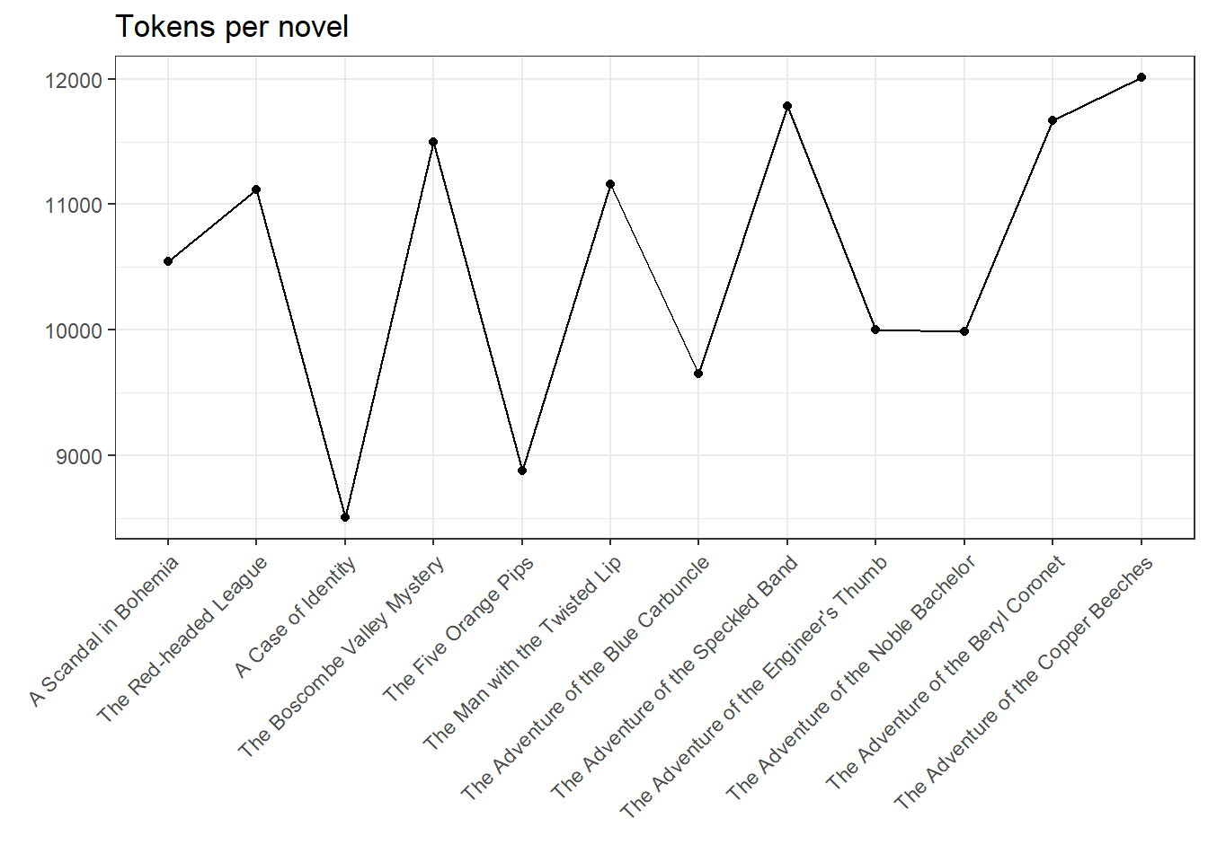
ggplot(my.corpus.stats, aes(Text, Types, group = 1)) + geom_line() + geom_point() + theme(axis.text.x = element_text(angle = 45, vjust = 1, hjust = 1)) + ggtitle("Types per novel") + xlab("") + ylab("")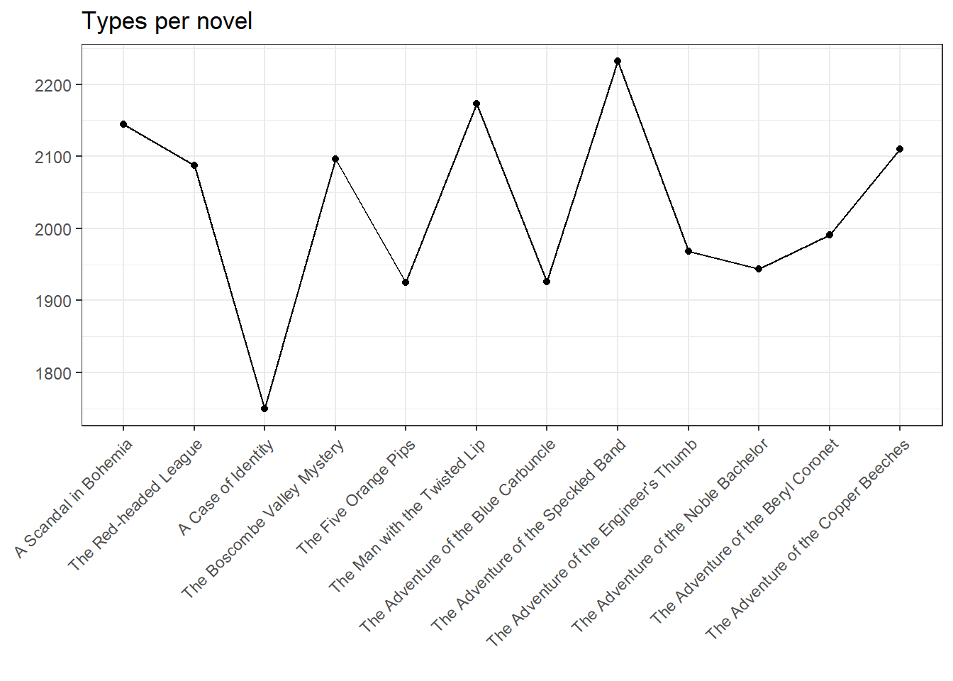
ggplot(my.corpus.stats, aes(Text, Sentences, group = 1)) + geom_line() + geom_point() + theme(axis.text.x = element_text(angle = 45, vjust = 1, hjust = 1)) + ggtitle("Sentences per novel") + xlab("") + ylab("")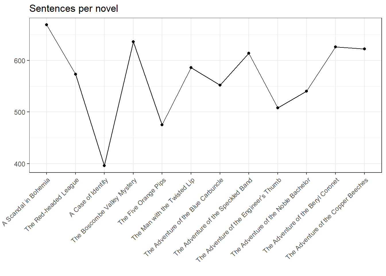
ggplot(my.corpus.stats, aes(Tokens, Types, group = 1, label = Textno)) + geom_smooth(method = "lm", se = FALSE) + geom_text(check_overlap = T) + ggtitle("Type-Token-Ratio (TTR) per novel")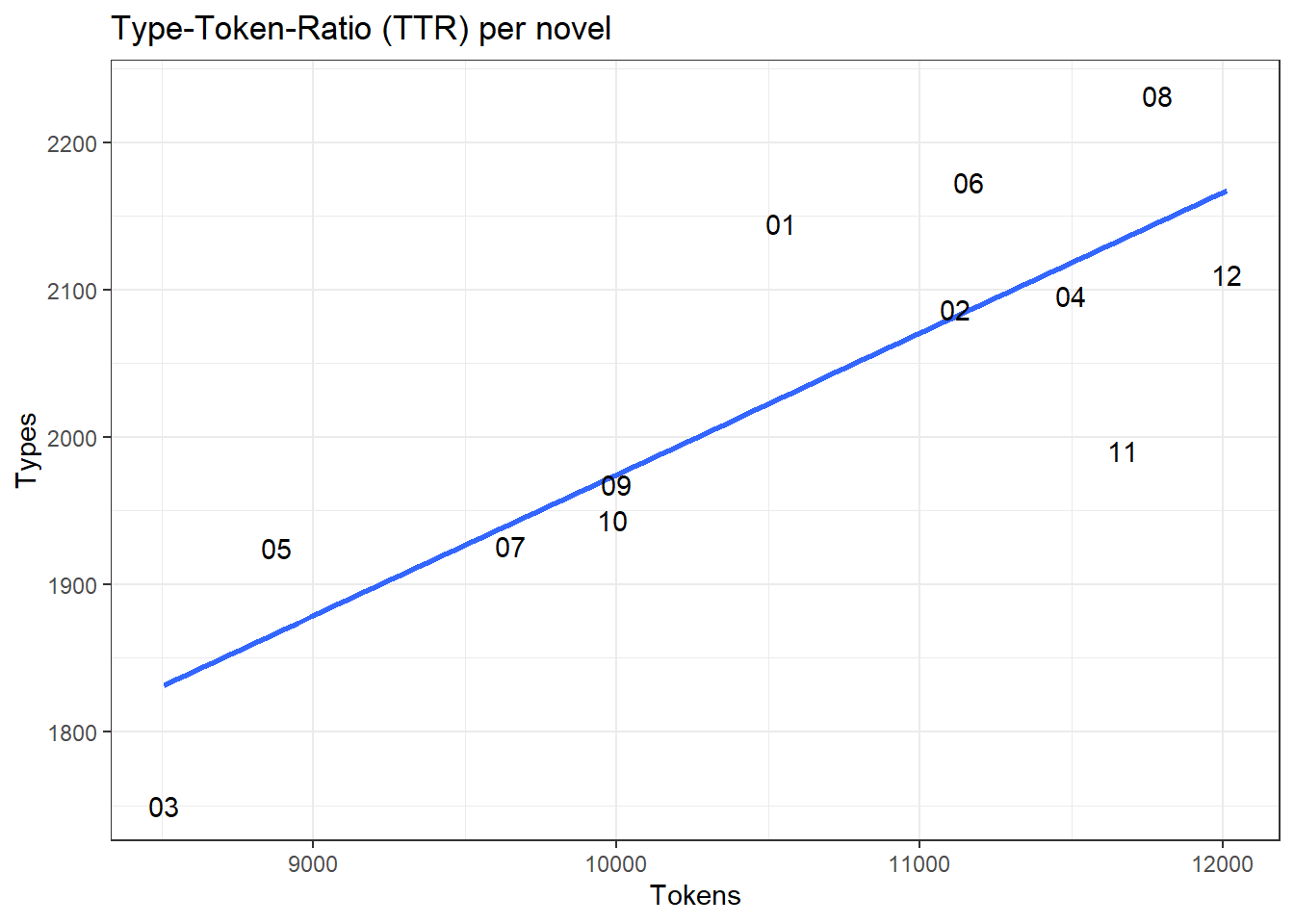
These charts are not very informative at first glance. They merely prove that the stories ‘A Case of Identity’ and (to a lesser extent) ‘The Five Orange Pips’ are significantly shorter than the other texts, which is reflected on all three levels (tokens, types, sentences). However, the type-token relation is somewhat more interesting: while three novels (i.e., numbers 3, 11, and 12) each have a TTR below average, another four are above the linear relation (1, 5, 6, and 8), with the remaining six novels corresponding fairly exact to the average. Thereby, the TTR can be used to draw conclusions about information density – we’ll come back to that later.
Working with corpora
Corpora in quanteda are very easy to create, reshape, and enrich with additional metadata. Metadata can in turn be used to filter the corpus according to specific criteria. The following call extracts the first 500 words of the first novel.
str_sub(my.corpus[1], start = 1, end = 500)## [1] "A Scandal in Bohemia\n\n To Sherlock Holmes she is always the woman. I have seldom\nheard him mention her under any other name. In his eyes she\neclipses and predominates the whole of her sex. It was not that\nhe felt any emotion akin to love for Irene Adler. All emotions,\nand that one particularly, were abhorrent to his cold, precise but\nadmirably balanced mind. He was, I take it, the most perfect\nreasoning and observing machine that the world has seen, but as\na lover he would have placed himself i"Each text can therefore be called up and also changed on the basis of its indexing (e.g. my.corpus[1] for the first text). The same works with the function texts – the way to get the index is simply the short form of texts(my.corpus)[1].
By means of corpus_reshape, a corpus can be transformed in such a way that each sentence results in its own document. Alternative arguments are “paragraphs” and “documents” (so a sentence corpus can be restored to its initial state). The creation of sentence corpora is of interest for sentiment analysis and supervised machine learning.
The label of the example consists of the variable docname and an appended number (1 for the first sentence).
my.corpus.sentences <- corpus_reshape(my.corpus, to = "sentences")
my.corpus.sentences[200]
## A Scandal in Bohemia.200
## "\"Then I fail to follow your Majesty."With corpus_sample(), a random sample may be drawn from a corpus. We apply the function here to the sentence corpus to retrieve one random sentence.
example.sentence <- corpus_sample(my.corpus.sentences, size = 1)
example.sentence[1]
## A Scandal in Bohemia.184
## "In this case I found her biography sandwiched in between that of a Hebrew rabbi and that of a staff-commander who had written a monograph upon the deep-sea fishes."Using corpus_subset, a corpus can finally be filtered by metadata. Here, this is done using the newly created binary variable LongSentence, which is TRUE if a set contains >= 25 tokens). In this way a partial corpus can be formed in which only longer sentences are contained. The example is only intended to illustrate that using the functions provided by quanteda, numerous steps can be taken to clean up our corpora.
docvars(my.corpus.sentences, "CharacterCount") <- ntoken(my.corpus.sentences)
docvars(my.corpus.sentences, "LongSentence") <- ntoken(my.corpus.sentences) >= 25
my.corpus.sentences_long <- corpus_subset(my.corpus.sentences, LongSentence == TRUE)
my.corpus.sentences_long[1:3]
## A Scandal in Bohemia.6
## "He was, I take it, the most perfect reasoning and observing machine that the world has seen, but as a lover he would have placed himself in a false position."
## A Scandal in Bohemia.9
## "But for the trained teasoner to admit such intrusions into his own delicate and finely adjusted temperament was to introduce a distracting factor which might throw a doubt upon all his mental results."
## A Scandal in Bohemia.10
## "Grit in a sensitive instrument, or a crack in one of his own high-power lenses, would not be more disturbing than a strong emotion in a nature such as his."One of quanteda’s greatest strengths is its ability to work with existing metadata variables (e.g. author, source, category, timestamp) and metadata variables created in-house (e.g. topic, sentiment). We will make great use of this feature in the following we often chapters, where we filter or group on the basis of metadata. Finally, corpora can also be split according to certain criteria using corpus_segment().
Tokenization
Tokenization refers to the splitting of a text into running words or so-called N-grams (i.e., sequences of several words in succession). The function tokens realizes the tokenization of a corpus in quanteda. In addition, tokens also understands countless arguments for removing certain features.
my.tokens <- tokens(my.corpus) %>% as.list()
head(my.tokens$`A Scandal in Bohemia`, 12)
## [1] "A" "Scandal" "in" "Bohemia" "To" "Sherlock"
## [7] "Holmes" "she" "is" "always" "the" "woman"Using the tokens function, the text can also be split into N-grams (the multi-word sequences, each consisting of N words) using the argument ngrams. In the following example, bigrams (or 2-grams, for that matter, although nobody refers to them that way) from the beginning of the first text are displayed, and then all sequences of one, two, or three terms are extracted (by using head we see only trigrams, but there are also shorter sequences).
my.tokens <- tokens(my.corpus, ngrams = 3) %>% as.list()
head(my.tokens$`A Scandal in Bohemia`)
## [1] "A_Scandal_in" "Scandal_in_Bohemia" "in_Bohemia_To"
## [4] "Bohemia_To_Sherlock" "To_Sherlock_Holmes" "Sherlock_Holmes_she"It is also helpful to be able to remove or retain certain terms during tokenization.
my.tokens <- tokens(my.corpus)
tokens.retained <- tokens_select(my.tokens, c("holmes", "watson")) %>% as.list()
head(tokens.retained$`A Scandal in Bohemia`)
## [1] "Holmes" "Holmes" "Holmes" "Holmes" "Watson" "Watson"tokens.removed <- tokens_remove(my.tokens, c("Sherlock", "in", "is", "the")) %>% as.list()
head(tokens.removed$`A Scandal in Bohemia`)## [1] "A" "Scandal" "Bohemia" "To" "Holmes" "she"As already mentioned, the tokens function accepts a number of arguments that can be used to exclude or retain whole classes of strings (numbers, punctuation, symbols …). First, numbers, punctuation and symbols will be removed, then tokens_tolower will be used to convert all words to lower case and then the words “sherlock” and “holmes” will be removed, as well as a number of english stop words.
my.tokens <- tokens(my.corpus, remove_numbers = TRUE, remove_punct = TRUE, remove_symbols = TRUE) %>%
  tokens_tolower() %>%
  tokens_remove(c(stopwords("english"), "sherlock", "holmes")) %>%
  as.list()
head(my.tokens$`A Scandal in Bohemia`)
## [1] "scandal" "bohemia" "always" "woman" "seldom" "heard"The result is very similar to the kind of data often used in procedures such as the use of lexicons, supervised machine learning and the calculation of topic models. The removal of stop words and other steps cause syntactic information to be lost (e.g., it is no longer possible to understand who is doing what with whom, or how the text is structured argumentatively or narratively). However, this information is not necessarily relevant in the bag-of-words approach, which is the most commonly used approach in automated content analysis.
Although the steps described in this section are useful in individual cases, they are practically never applied in the following chapters because the data are already available there as quanteda corpora where such preprocessing has already been applied. The tokenization is also implicitly applied as soon as a document feature matrix (DFM, see below) is created.
Document Feature Matrices (DFMs)
We now come to a central data structure of quanteda, which, in contrast to the previously introduced functions, occurs in practically every project – the Document Feature Matrix (DFM). A DFM is a table, which depicts texts as rows and individual words as columns; in each cell, then, the frequencies of a given word in a given text is noted. Usually, the DFM (or several ones, if necessary) is (are) calculated directly after a corpus has been created. Consequently, information about where a word occurs in a text is lost (that’s why it’s referred to as bag-of-words approach, where DFMs are not-positional in contrast to the actual corpus). Whenever we are interested in the relationship of words to texts (and vice versa), we calculate a DFM.
my.dfm <- dfm(my.corpus, remove_numbers = TRUE, remove_punct = TRUE, remove_symbols = TRUE, remove = stopwords("english"))
my.dfm
## Document-feature matrix of: 12 documents, 8,489 features (79.1% sparse).Importantly, the tokens() function, which we are already familiar with, is implicitly used here to remove (or possibly retain) certain features. Many things work with DFMs just like they work when creating a corpus. For example, the functions ndoc() and nfeat() count documents and features (words, in our case).
ndoc(my.dfm)## [1] 12nfeat(my.dfm)## [1] 8489Using the functions docnames() and featnames(), we can also display the names of the documents and features.
head(docnames(my.dfm))## [1] "A Scandal in Bohemia" "The Red-headed League"
## [3] "A Case of Identity" "The Boscombe Valley Mystery"
## [5] "The Five Orange Pips" "The Man with the Twisted Lip"head(featnames(my.dfm), 50)## [1] "scandal" "bohemia" "sherlock" "holmes"
## [5] "always" "woman" "seldom" "heard"
## [9] "mention" "name" "eyes" "eclipses"
## [13] "predominates" "whole" "sex" "felt"
## [17] "emotion" "akin" "love" "irene"
## [21] "adler" "emotions" "one" "particularly"
## [25] "abhorrent" "cold" "precise" "admirably"
## [29] "balanced" "mind" "take" "perfect"
## [33] "reasoning" "observing" "machine" "world"
## [37] "seen" "lover" "placed" "false"
## [41] "position" "never" "spoke" "softer"
## [45] "passions" "save" "gibe" "sneer"
## [49] "admirable" "things"The tabular view best illustrates what a DFM actually does as a text-word matrix. Importantly, the reported sparsity of a DFM describes the proportion of empty cells (i.e., words that occur only in very few texts). As can easily be deduced, DFMs quickly become very large. Fortunately, quanteda takes advantage of a number of features from other packages that are invisible to the user to address this problem.
head(my.dfm, n = 12, nf = 10) # Features/texts as a matrix## Document-feature matrix of: 12 documents, 10 features (30.8% sparse).
## 12 x 10 sparse Matrix of class "dfm"
## features
## docs scandal bohemia sherlock holmes
## A Scandal in Bohemia 4 8 11 47
## The Red-headed League 0 0 10 51
## A Case of Identity 0 2 7 46
## The Boscombe Valley Mystery 1 0 10 43
## The Five Orange Pips 1 0 10 25
## The Man with the Twisted Lip 0 0 10 28
## The Adventure of the Blue Carbuncle 0 0 10 34
## The Adventure of the Speckled Band 0 0 9 55
## The Adventure of the Engineer's Thumb 0 0 5 12
## The Adventure of the Noble Bachelor 1 0 7 34
## The Adventure of the Beryl Coronet 4 0 3 26
## The Adventure of the Copper Beeches 0 1 2 42
## features
## docs always woman seldom heard mention
## A Scandal in Bohemia 5 12 3 8 1
## The Red-headed League 5 0 0 15 0
## A Case of Identity 7 10 0 5 0
## The Boscombe Valley Mystery 5 1 0 10 0
## The Five Orange Pips 5 1 0 5 1
## The Man with the Twisted Lip 4 5 0 8 0
## The Adventure of the Blue Carbuncle 5 0 1 3 0
## The Adventure of the Speckled Band 8 5 1 20 0
## The Adventure of the Engineer's Thumb 0 6 1 11 0
## The Adventure of the Noble Bachelor 3 8 0 11 0
## The Adventure of the Beryl Coronet 3 5 0 12 0
## The Adventure of the Copper Beeches 7 8 0 5 0
## features
## docs name
## A Scandal in Bohemia 6
## The Red-headed League 6
## A Case of Identity 1
## The Boscombe Valley Mystery 3
## The Five Orange Pips 5
## The Man with the Twisted Lip 4
## The Adventure of the Blue Carbuncle 10
## The Adventure of the Speckled Band 6
## The Adventure of the Engineer's Thumb 3
## The Adventure of the Noble Bachelor 6
## The Adventure of the Beryl Coronet 8
## The Adventure of the Copper Beeches 4At first glance, you will notice that the words “sherlock” and “holmes” are not very distinctive in all novels, which is why we might want to add them to the stop words for this corpus – they simply do not provide much additional insight.
Looking at the DFM sorted by prevalent features is usually more informative than inspecting the features in the order of their occurance.
head(dfm_sort(my.dfm, decreasing = TRUE, margin = "both"), n = 12, nf = 10) ## Document-feature matrix of: 12 documents, 10 features (0.0% sparse).
## 12 x 10 sparse Matrix of class "dfm"
## features
## docs said upon holmes one man mr little
## The Adventure of the Speckled Band 44 41 55 33 11 5 17
## The Adventure of the Copper Beeches 47 33 42 36 34 44 37
## The Boscombe Valley Mystery 37 42 43 31 41 24 25
## The Man with the Twisted Lip 28 54 28 36 30 20 21
## The Adventure of the Beryl Coronet 45 33 26 32 27 20 22
## The Red-headed League 51 50 51 29 25 55 25
## A Scandal in Bohemia 33 25 47 27 23 9 14
## The Adventure of the Engineer's Thumb 47 38 12 33 17 11 25
## The Adventure of the Noble Bachelor 33 29 34 31 10 17 26
## The Adventure of the Blue Carbuncle 43 38 34 38 37 17 24
## The Five Orange Pips 32 47 25 29 19 3 5
## A Case of Identity 45 35 46 17 16 50 28
## features
## docs now see may
## The Adventure of the Speckled Band 21 22 19
## The Adventure of the Copper Beeches 18 17 21
## The Boscombe Valley Mystery 16 24 19
## The Man with the Twisted Lip 27 18 15
## The Adventure of the Beryl Coronet 29 20 25
## The Red-headed League 14 23 8
## A Scandal in Bohemia 17 15 21
## The Adventure of the Engineer's Thumb 16 16 9
## The Adventure of the Noble Bachelor 16 16 18
## The Adventure of the Blue Carbuncle 33 27 7
## The Five Orange Pips 12 16 24
## A Case of Identity 15 15 11The topfeatures() function counts features in the entire DFM. The function textstat_frequency() additionally supplies the rank, the number of documents in which the feature occurs (docfreq) as well as metadata, which was used for filtering during the count (textstat_frequncy is to be preferred to topfeatures).
topfeatures(my.dfm) # basic word frequencies## said upon holmes one man mr little now see may
## 485 465 443 372 290 275 269 234 229 197word.frequencies <- textstat_frequency(my.dfm) # more elaborate frequencies
head(word.frequencies)Working with DFMs
As has already been indicated, DFMs can be easily sorted by document and feature frequencies using dfm_sort.
head(dfm_sort(my.dfm, decreasing = TRUE, margin = "both"), n = 12, nf = 10) ## Document-feature matrix of: 12 documents, 10 features (0.0% sparse).
## 12 x 10 sparse Matrix of class "dfm"
## features
## docs said upon holmes one man mr little
## The Adventure of the Speckled Band 44 41 55 33 11 5 17
## The Adventure of the Copper Beeches 47 33 42 36 34 44 37
## The Boscombe Valley Mystery 37 42 43 31 41 24 25
## The Man with the Twisted Lip 28 54 28 36 30 20 21
## The Adventure of the Beryl Coronet 45 33 26 32 27 20 22
## The Red-headed League 51 50 51 29 25 55 25
## A Scandal in Bohemia 33 25 47 27 23 9 14
## The Adventure of the Engineer's Thumb 47 38 12 33 17 11 25
## The Adventure of the Noble Bachelor 33 29 34 31 10 17 26
## The Adventure of the Blue Carbuncle 43 38 34 38 37 17 24
## The Five Orange Pips 32 47 25 29 19 3 5
## A Case of Identity 45 35 46 17 16 50 28
## features
## docs now see may
## The Adventure of the Speckled Band 21 22 19
## The Adventure of the Copper Beeches 18 17 21
## The Boscombe Valley Mystery 16 24 19
## The Man with the Twisted Lip 27 18 15
## The Adventure of the Beryl Coronet 29 20 25
## The Red-headed League 14 23 8
## A Scandal in Bohemia 17 15 21
## The Adventure of the Engineer's Thumb 16 16 9
## The Adventure of the Noble Bachelor 16 16 18
## The Adventure of the Blue Carbuncle 33 27 7
## The Five Orange Pips 12 16 24
## A Case of Identity 15 15 11Furthermore, certain features of a DFM can be specifically selected using dfm_select.
dfm_select(my.dfm, pattern = "lov*")## Document-feature matrix of: 12 documents, 7 features (67.9% sparse).
## 12 x 7 sparse Matrix of class "dfm"
## features
## docs love lover lovely loves loved
## A Scandal in Bohemia 5 1 1 1 1
## The Red-headed League 1 0 0 0 0
## A Case of Identity 2 0 0 0 0
## The Boscombe Valley Mystery 1 0 1 0 1
## The Five Orange Pips 1 0 0 0 0
## The Man with the Twisted Lip 0 0 0 0 0
## The Adventure of the Blue Carbuncle 2 0 0 0 0
## The Adventure of the Speckled Band 1 0 1 0 0
## The Adventure of the Engineer's Thumb 1 0 0 0 0
## The Adventure of the Noble Bachelor 1 2 1 0 0
## The Adventure of the Beryl Coronet 3 4 0 2 3
## The Adventure of the Copper Beeches 0 0 1 1 0
## features
## docs lovers loving
## A Scandal in Bohemia 0 0
## The Red-headed League 0 0
## A Case of Identity 1 0
## The Boscombe Valley Mystery 0 0
## The Five Orange Pips 0 0
## The Man with the Twisted Lip 0 0
## The Adventure of the Blue Carbuncle 0 0
## The Adventure of the Speckled Band 0 0
## The Adventure of the Engineer's Thumb 0 0
## The Adventure of the Noble Bachelor 0 1
## The Adventure of the Beryl Coronet 0 2
## The Adventure of the Copper Beeches 0 0The function dfm_wordstem() reduces words to their root form. This function currently exists in quanteda only for English and is not very reliable, which is well illustrated in the following issue (‘holm’ is not a root word). We will come back to language-specific information, though, in other chapters.
my.dfm.stemmed <- dfm_wordstem(my.dfm)
topfeatures(my.dfm.stemmed)
## said upon holm one man mr littl see now come
## 485 465 460 383 304 275 269 253 234 207As with word frequencies in corpora, the weighting of a DFM according to relative word frequencies and methods such as TF-IDF often makes sense. The weighting of a DFM always works based on the word-text relation, which is why topfeatures() in combination with dfm_weight() produces strange results. Relative frequencies and TF-IDF are only meaningful contrastively within the text in a corpus (here for ‘A Scandal in Bohemia’), since for the whole corpus’ relative frequency equals its absolute frequency.
my.dfm.proportional <- dfm_weight(my.dfm, scheme = "propmax")
convert(my.dfm.proportional, "data.frame")
In the second example, we see that ‘A Scandal in Bohemia’ has a slightly higher proportion of citations of the word ‘holmes’ than is the case in the whole corpus. A little more about that later.
The weighting approaches Propmax and TF-IDF provide relevant word metrics, for example for the determination of stop words. Propmax scales the word frequency relative to the most frequent word (here ‘holmes’).
my.dfm.propmax <- dfm_weight(my.dfm, scheme = "propmax")
topfeatures(my.dfm.propmax[1,])
## holmes said one upon man may
## 1.0000000 0.7021277 0.5744681 0.5319149 0.4893617 0.4468085
## photograph street know now
## 0.4042553 0.3829787 0.3829787 0.3617021Functionally, TF-IDF and the Keyness approach (introduced later) are similar – both find particularly distinctive terms.
my.dfm.tfidf <- dfm_tfidf(my.dfm)
topfeatures(my.dfm.tfidf)
## simon rucastle mccarthy coronet lestrade hosmer clair k
## 42.08807 36.69216 34.53380 29.13789 28.01345 24.82117 24.82117 22.66281
## hunter wilson
## 22.66281 21.58362Finally, you can create a reduced document feature matrix with dfm_trim(). This makes sense if one assumes, for example, that only terms that occur at least X times in the entire body play a role. A minimum number or maximum number of documents in which a term must or may occur can also be determined. Both filter options can also be used proportionally – below, we first extract those features found in at least 11 novels, and then those in the 95th frequency percentile (i.e., the top 5% of all features).
my.dfm.trim <- dfm_trim(my.dfm, min_docfreq = 11)
head(my.dfm.trim, n = 12, nf = 10)
## Document-feature matrix of: 12 documents, 10 features (2.5% sparse).
## 12 x 10 sparse Matrix of class "dfm"
## features
## docs sherlock holmes always heard name
## A Scandal in Bohemia 11 47 5 8 6
## The Red-headed League 10 51 5 15 6
## A Case of Identity 7 46 7 5 1
## The Boscombe Valley Mystery 10 43 5 10 3
## The Five Orange Pips 10 25 5 5 5
## The Man with the Twisted Lip 10 28 4 8 4
## The Adventure of the Blue Carbuncle 10 34 5 3 10
## The Adventure of the Speckled Band 9 55 8 20 6
## The Adventure of the Engineer's Thumb 5 12 0 11 3
## The Adventure of the Noble Bachelor 7 34 3 11 6
## The Adventure of the Beryl Coronet 3 26 3 12 8
## The Adventure of the Copper Beeches 2 42 7 5 4
## features
## docs eyes whole felt one cold
## A Scandal in Bohemia 9 4 2 27 2
## The Red-headed League 10 9 4 29 1
## A Case of Identity 6 3 3 17 1
## The Boscombe Valley Mystery 6 2 0 31 1
## The Five Orange Pips 5 2 2 29 1
## The Man with the Twisted Lip 11 3 2 36 2
## The Adventure of the Blue Carbuncle 2 0 4 38 5
## The Adventure of the Speckled Band 11 1 2 33 3
## The Adventure of the Engineer's Thumb 4 4 4 33 1
## The Adventure of the Noble Bachelor 4 4 3 31 2
## The Adventure of the Beryl Coronet 10 6 4 32 1
## The Adventure of the Copper Beeches 9 7 2 36 1my.dfm.trim <- dfm_trim(my.dfm, min_termfreq = 0.95, termfreq_type = "quantile")
head(my.dfm.trim, n = 12, nf = 10) ## Document-feature matrix of: 12 documents, 10 features (4.17% sparse).
## 12 x 10 sparse Matrix of class "dfm"
## features
## docs sherlock holmes always woman heard
## A Scandal in Bohemia 11 47 5 12 8
## The Red-headed League 10 51 5 0 15
## A Case of Identity 7 46 7 10 5
## The Boscombe Valley Mystery 10 43 5 1 10
## The Five Orange Pips 10 25 5 1 5
## The Man with the Twisted Lip 10 28 4 5 8
## The Adventure of the Blue Carbuncle 10 34 5 0 3
## The Adventure of the Speckled Band 9 55 8 5 20
## The Adventure of the Engineer's Thumb 5 12 0 6 11
## The Adventure of the Noble Bachelor 7 34 3 8 11
## The Adventure of the Beryl Coronet 3 26 3 5 12
## The Adventure of the Copper Beeches 2 42 7 8 5
## features
## docs name eyes whole felt one
## A Scandal in Bohemia 6 9 4 2 27
## The Red-headed League 6 10 9 4 29
## A Case of Identity 1 6 3 3 17
## The Boscombe Valley Mystery 3 6 2 0 31
## The Five Orange Pips 5 5 2 2 29
## The Man with the Twisted Lip 4 11 3 2 36
## The Adventure of the Blue Carbuncle 10 2 0 4 38
## The Adventure of the Speckled Band 6 11 1 2 33
## The Adventure of the Engineer's Thumb 3 4 4 4 33
## The Adventure of the Noble Bachelor 6 4 4 3 31
## The Adventure of the Beryl Coronet 8 10 6 4 32
## The Adventure of the Copper Beeches 4 9 7 2 36Visualizing DFMs
DFMs can also be represented as a word cloud of the most common terms.
textplot_wordcloud(my.dfm, min_size = 1, max_size = 5, max_words = 100)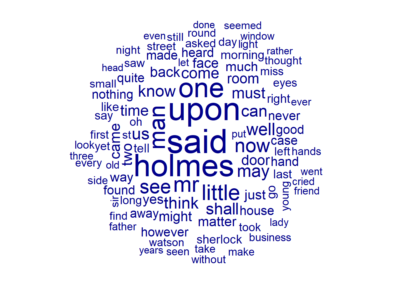
The comparison is also more interesting than the presentation of the entire corpus. The following plot shows the most distinctive terms according to TF-IDF for four novels, where the color indicates the respective novel. The fact that the word size in the plot does not indicate the absolute frequency but the TF-IDF value makes such a plot useful for direct comparison.
textplot_wordcloud(my.dfm[1:4,], color = brewer.pal(4, "Set1"), min_size = 0.2, max_size = 4, max_words = 50, comparison = TRUE)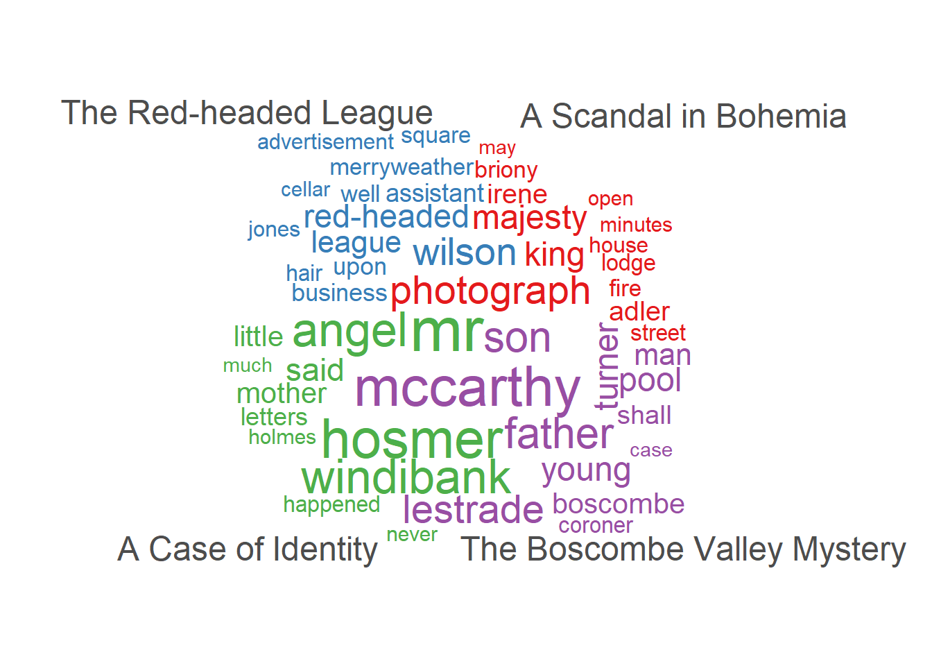
Things to remember about quanteda basics
The following characteristics of corpora and DFMs should be kept in mind:
- a corpus consists of texts (or tweets, comments …) and metadata
- a corpus is positional, a DFM is non-positional
- in most projects you want one corpus to contain all your data and generate many DFMs from that
- the rows of a DFM can contain any unit on which you can aggregates documents
- the columns of a DFM are any unit on which you can aggregate features