Automated Content Analysis with R
Supervised machine learning
Cornelius Puschmann & Mario Haim
Supervised machine learning is a process to automatically extract rules from a coded dataset, which subsequently can be applied to a thus far not coded dataset. Typically, a conventional manual content analysis is carried out first, within which human coders annotate a sample of texts to one or more categories on the basis of a codebook. The features of these texts are then evaluated to “learn” rules for annotation of new texts. Oftentimes, machine learning is based on complete texts; however, it could build on certain terms only, or even on N-grams, or more complex patterns, such as different sentence types.
Due to the initially coded dataset, rule-extraction is guided by this “gold standard.” This is why it is called supervised learning, because it is possible to check the quality of the automated classification on the basis of already annotated data. Hence, a central advantage of supervised learning is that, compared to human coders, the computer is both faster and more reliable – given, that only reliable rules can be derived from the information used for learning (the so-called training data). If this is not the case, the results are anything but impressive.
What can supervised machine learning with regard to text data be used for? In essence, the procedures described below are relevant for at least four different applications:
- automated classification of not yet annotated texts in combination with an already performed manual content analysis;
- validation of a manual content analysis;
- classification based on categories that are not actually classic content analysis categories, but can be used as such (such as a newspaper article section);
- to gain an understanding of which factors contribute to a classification result and how
A number of algorithms are available to perform such analyses. Basically, we always need an already annotated data set to develop a model, where both the quality of the annotation and the size of the data set must be sufficient to enable reliable automation. Again, we start by loading the necessary libraries.
if(!require("quanteda")) {install.packages("quanteda"); library("quanteda")}
if(!require("tidyverse")) {install.packages("tidyverse"); library("tidyverse")}
theme_set(theme_bw())
Load the Reddit corpus
We start with the same corpus that we already used in chapter 3 on ~20,000 comments posted to two subreddits, ‘science’ and ‘syriancivilwar’.
load("data/reddit.RData")
reddit.corpus
## Corpus consisting of 20,603 documents and 16 docvars.Calculate and trim a DFM
We then calculate our document-term matrix and apply some preprocessing in the form of cleaning. That is, we ask quanteda to remove numbers and punctuation, erase URLs and also remove various stopwords (i.e., the most common words in a language). For the actual machine learning, we also reduce the data included through the dfm_trim() function. Note, however, that it is okay for the training with complete data to run for several hours.
dfm.reddit <- dfm(reddit.corpus, remove_numbers = TRUE, remove_punct = TRUE, remove_url = TRUE, remove = c(stopwords("english"), "people", "time", "day", "years", "just", "really", "one", "can", "like", "go", "get", "gt", "amp", "now", "get", "much", "many", "every", "lot", "even", "also"))
dfm.reddit
## Document-feature matrix of: 20,603 documents, 30,838 features (99.9% sparse).dfm.reddit.trim <- dfm_trim(dfm.reddit, min_docfreq = 0.0005, docfreq_type = "prop") # about 15 docs
dfm.reddit.trim## Document-feature matrix of: 20,603 documents, 4,663 features (99.7% sparse).Apply the Naive Bayes (NB) classifier
To actually train our model, we need to implement a respective algorithm. There is a wide variety available, the more prominent of which might be naive-bayes classifier, support vector machines, or random-forest algorithms. A lot of these algorithms require own packages (and some also very heavy computational ressources). We thus rely on Naive Bayes here, because it’s included in quanteda through the textmodel_nb() function and because it comparably cheap on computational ressources.
model.NB <- textmodel_nb(dfm.reddit.trim, reddit.stats$subreddit, prior = "docfreq")

"First 20 predicted categories (should all be science, a few are wrong)"
## [1] "First 20 predicted categories (should all be science, a few are wrong)"head(as.character(predict(model.NB)), 20)## [1] "science" "syriancivilwar" "science" "science"
## [5] "science" "syriancivilwar" "science" "science"
## [9] "science" "science" "science" "science"
## [13] "science" "science" "science" "science"
## [17] "science" "science" "science" "science""Percentage of NB classifier predictions that are correct"## [1] "Percentage of NB classifier predictions that are correct"prop.table(table(predict(model.NB) == reddit.stats$subreddit))*100##
## FALSE TRUE
## 13.16799 86.83201What we are presented with, are the “results,” which actually refers to the automatically annotated documents after training a model. In other words, the results show how the trained model performs. As such, we can see that among the first 20 documents, two have been classified as “syriancivilwar” while in fact all should have been classified as “science” (i.e., 90% were correct). Scaled up to all ~20.000 documents, this is also almost the share of documents classified correctly. Note, that the number might change for your local run of the script due to model-training differences.
That said, is that a good result? For an easy estimation of the quality of our model, we can simply compare it to a randomly annotated sample (where we keep the correct distribution of categories). As this is a dichotomous decision, by chance means literally a coin toss. In other words, our Naive Bayes classification is pretty okay.
prop.table(table(sample(predict(model.NB)) == reddit.stats$subreddit))*100##
## FALSE TRUE
## 49.94904 50.05096Next, we can look at the significant terms, that led the model to decide on either category.
nb.terms <- as.data.frame(t(model.NB$PwGc)) %>%
  rownames_to_column("Word") %>%
  gather(Subreddit, Association, -Word) %>%
  arrange(Subreddit, desc(Association)) %>%
  group_by(Subreddit) %>%
  mutate(Rank = row_number()) %>%
  filter(Rank <= 25)
ggplot(filter(nb.terms, Subreddit == "science"), aes(reorder(Word, Rank), Association)) + geom_bar(stat = "identity") + theme(axis.text.x = element_text(angle = 45, hjust = 1)) + xlab("") + ylab("") + ggtitle("Subreddit science")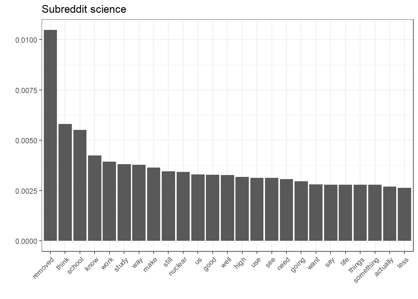
ggplot(filter(nb.terms, Subreddit == "syriancivilwar"), aes(reorder(Word, Rank), Association)) + geom_bar(stat = "identity") + theme(axis.text.x = element_text(angle = 45, hjust = 1)) + xlab("") + ylab("") + ggtitle("Subreddit syriancivilwar")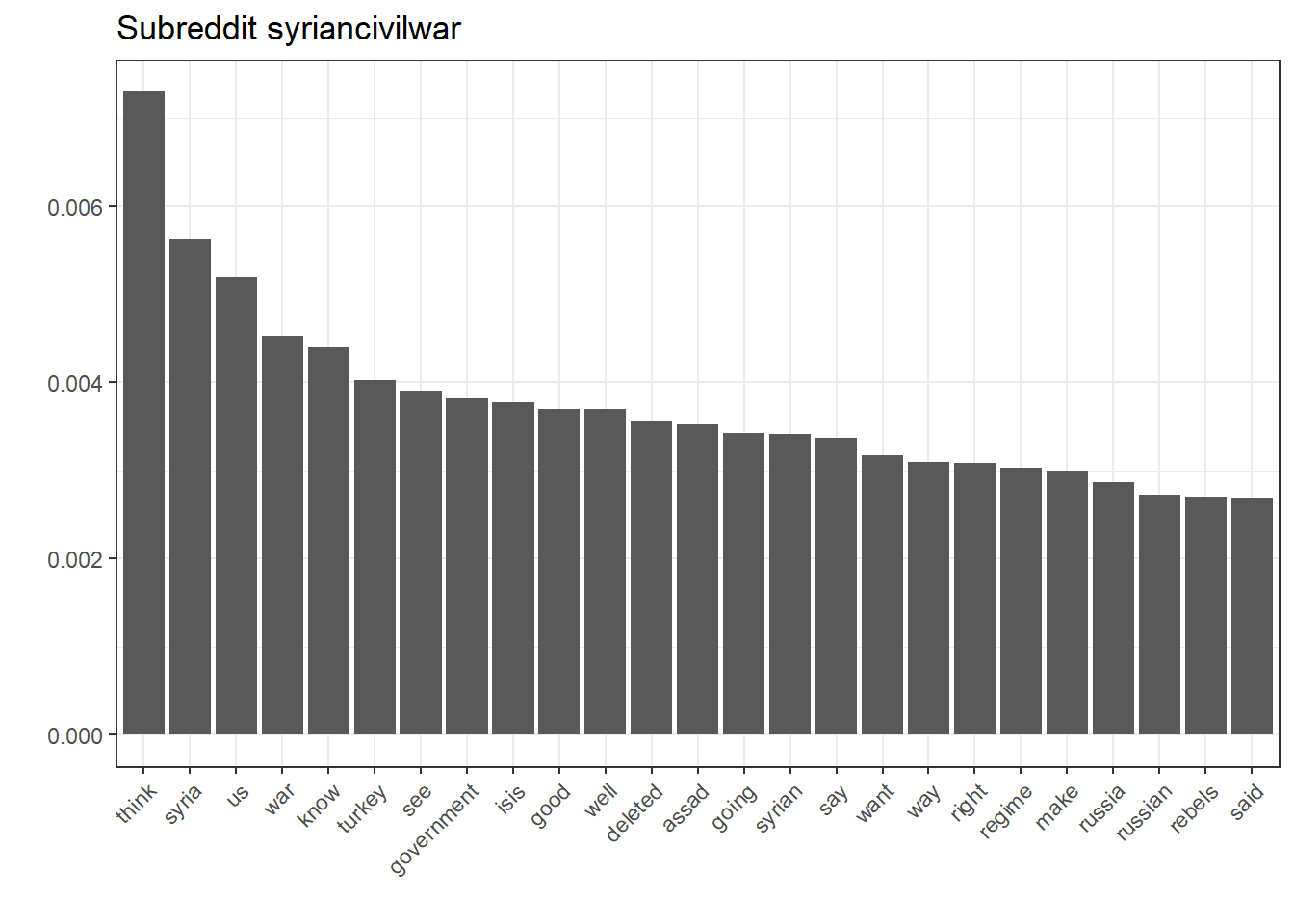
While this seems rather intuitive, it’s also a good way to inspect the kind-of black-box character that machine-learnt models depict.
Load the Trump/Clinton Twitter corpus
We continue with the Trump/Clinton corpus from chapter 3.
load("data/twitter/trumpclinton.RData")
trumpclinton.corpus
## Corpus consisting of 18,826 documents and 7 docvars.Again, we trim the newly created DFM to an easily managable size for this lecture purpose. However, for an actual work, keep in mind to train the model on all features.
dfm.trumpclinton <- dfm(trumpclinton.corpus, remove_numbers = TRUE, remove_symbols = TRUE, remove_punct = TRUE, remove_twitter = TRUE, remove_url = TRUE, remove = stopwords("en"))
dfm.trumpclinton
## Document-feature matrix of: 18,826 documents, 20,192 features (100.0% sparse).dfm.trumpclinton.trim <- dfm_trim(dfm.trumpclinton, min_docfreq = 0.0005, docfreq_type = "prop")
dfm.trumpclinton.trim## Document-feature matrix of: 18,826 documents, 2,498 features (99.7% sparse).And also again, we train a naive-bayes classifier and compare it to a randomly drawn sample.
model.NB <- textmodel_nb(dfm.trumpclinton.trim, trumpclinton.stats$Candidate, prior = "docfreq")
"First 20 predicted candidate variables (should all be Trump)"
## [1] "First 20 predicted candidate variables (should all be Trump)"head(as.character(predict(model.NB)), 20)## [1] "Trump" "Trump" "Trump" "Trump" "Trump" "Trump" "Trump" "Trump"
## [9] "Trump" "Trump" "Trump" "Trump" "Trump" "Trump" "Trump" "Trump"
## [17] "Trump" "Trump" "Trump" "Trump""Percentage of NB classifier predictions that are correct"## [1] "Percentage of NB classifier predictions that are correct"prop.table(table(predict(model.NB) == trumpclinton.stats$Candidate))*100##
## FALSE TRUE
## 7.633061 92.366939"Percentage of random chance predictions that are correct"## [1] "Percentage of random chance predictions that are correct"prop.table(table(sample(predict(model.NB)) == trumpclinton.stats$Candidate))*100##
## FALSE TRUE
## 48.24711 51.75289As this is a dichotomous decision as well, the random sample is close to 50% again. That said, our model is indeed pretty good which most likely is due a very clear distinction between the two candidates and their language used. Let’s inspect the most significant terms per candidate.
nb.terms <- as.data.frame(t(model.NB$PwGc)) %>%
  rownames_to_column("Word") %>%
  gather(Candidate, Association, -Word) %>%
  arrange(Candidate, desc(Association)) %>%
  group_by(Candidate) %>%
  mutate(Rank = row_number()) %>%
  filter(Rank <= 25)
ggplot(filter(nb.terms, Candidate == "Trump"), aes(reorder(Word, Rank), Association)) + geom_bar(stat = "identity") + theme(axis.text.x = element_text(angle = 45, hjust = 1)) + xlab("") + ylab("") + ggtitle("Key classifier features for Donald Trump")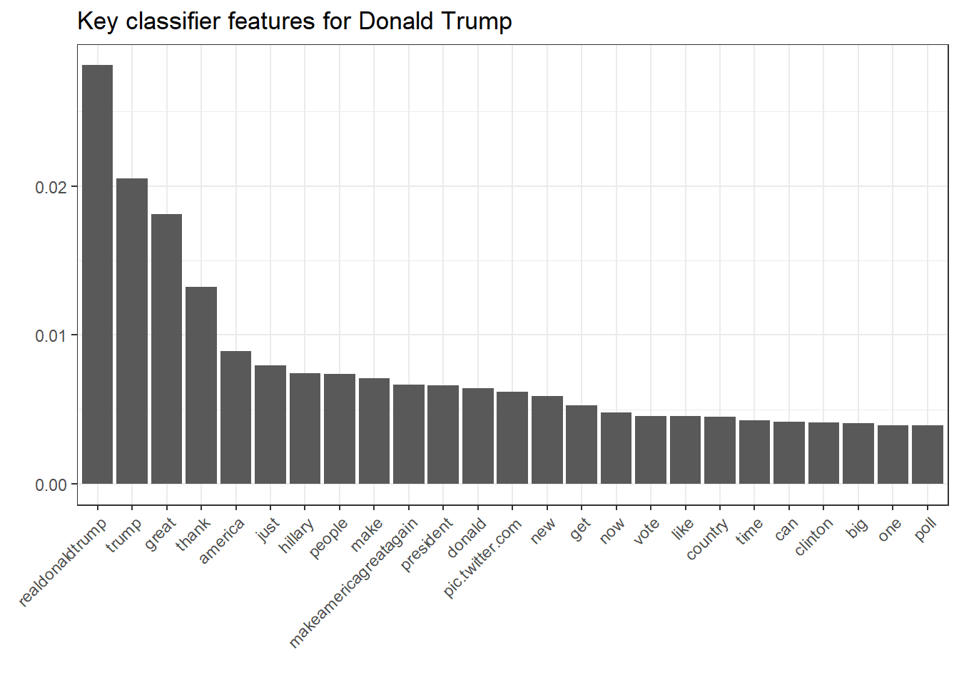
ggplot(filter(nb.terms, Candidate == "Clinton"), aes(reorder(Word, Rank), Association)) + geom_bar(stat = "identity") + theme(axis.text.x = element_text(angle = 45, hjust = 1)) + xlab("") + ylab("") + ggtitle("Key classifier features for Hillary Clinton")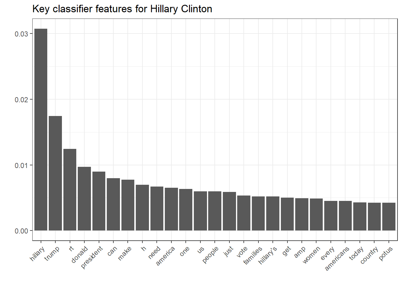
This underlines the last argument pretty well. While Clinton’s key features for classification reveal her campaign vocabulary and the stressed topics, Trump’s key features merely include topics but rather his famous superlative-savvy and direct language.
Multi-label categories
We turn to the New York Times Headline Corpus (Boydstun, 2013), which is a good basis for a first demonstration of supervised learning with more than two potential annotations. The basis of the analysis is the short summary of the article (not the full text), which can vary depending on the article. In addition, each line contains a number indicating the category to which the article was assigned.
load("data/nyt/nyt.korpus.RData")
as.data.frame(korpus.nyt.stats)
For easy interpretation of the results, we also import a simple data set containing the written names of the numerical topic codes.
labels.categories <- scan("data/nyt/majortopics2digits.txt", what = "char", sep = "\n", quiet = T)
labels.categories <- data.frame(Category = as.character(1:length(labels.categories)), Label = labels.categories, stringsAsFactors = F)
labels.categories
Once again we create a Document Feature Matrix (DFM). Since the texts are short summaries, hardly any features need to be removed.
nyt.dfm <- dfm(korpus.nyt, remove_numbers = TRUE, remove_punct = TRUE, remove = stopwords("english"))
nyt.dfm
## Document-feature matrix of: 30,862 documents, 16,499 features (100.0% sparse).This DFM is also reduced. The reduction is relatively strong here in order to be able to carry out the training process quickly with a satisfactory result. With a research project or a thesis, however, it is no problem if the calculation of the model takes several hours. Even with a correct analysis, it should be tested with which feature density an optimal result can be achieved.
nyt.dfm.trim <- dfm_trim(nyt.dfm, min_docfreq = 0.0005, docfreq_type = "prop")
nyt.dfm.trim
## Document-feature matrix of: 30,862 documents, 1,905 features (99.8% sparse).Again, we use quanteda’s textmodel_nb. This function expects a DFM, a list of labels (in our case, that’s “Topic_2digit”, which holds the numerical topic code), and an a-priori distribution (i.e., the frequency of occurrence of each category in the dataset). The codes displayed with the command head are therefore the predictions that the algorithm made for the test data based on its training.
modell.NB <- textmodel_nb(nyt.dfm.trim, korpus.nyt.stats$Topic_2digit, prior = "docfreq")
head(as.character(predict(modell.NB)))
## [1] "12" "28" "20" "16" "20" "10"head(as.character(korpus.nyt.stats$Topic_2digit))## [1] "12" "28" "20" "16" "20" "10"Again, we look at the correctly classified labels and the label classification by chance.
prop.table(table(predict(modell.NB) == korpus.nyt.stats$Topic_2digit))*100##
## FALSE TRUE
## 25.13771 74.86229prop.table(table(sample(predict(modell.NB)) == korpus.nyt.stats$Topic_2digit))*100##
## FALSE TRUE
## 89.80623 10.19377As we can see, the Bayesian classifier is not perfect, but it is much better than a random algorithm. It can also be used as an additional coder, especially if we take a closer look at which codes it performs particularly well or poorly. For this, we can display the match of the prediction with the human annotation by category. As we can see, the values are between 28% and 88%, the mean value (indicated by the blue line) is about 65%.
modell.NB.klassifikation <- bind_cols(korpus.nyt.stats, Classification = as.character(predict(modell.NB))) %>%
  mutate(Category = as.character(Topic_2digit)) %>%
  mutate(CorrectlyAnnotated = Classification == Category) %>%
  group_by(Category, CorrectlyAnnotated) %>%
  summarise(n = n()) %>%
  mutate(Share = n/sum(n)) %>%
  filter(CorrectlyAnnotated == TRUE) %>%
  left_join(labels.categories, by = "Category") %>%
  select(Category, Label, n, Share)
ggplot(modell.NB.klassifikation, aes(Label, Share)) + geom_bar(stat = "identity") + geom_hline(yintercept = mean(modell.NB.klassifikation$Share), color = "blue") + ylim(0, 1) + ggtitle("Share of correctly annotated texts applying a Bayes classifyer") + xlab("") + ylab("") + coord_flip()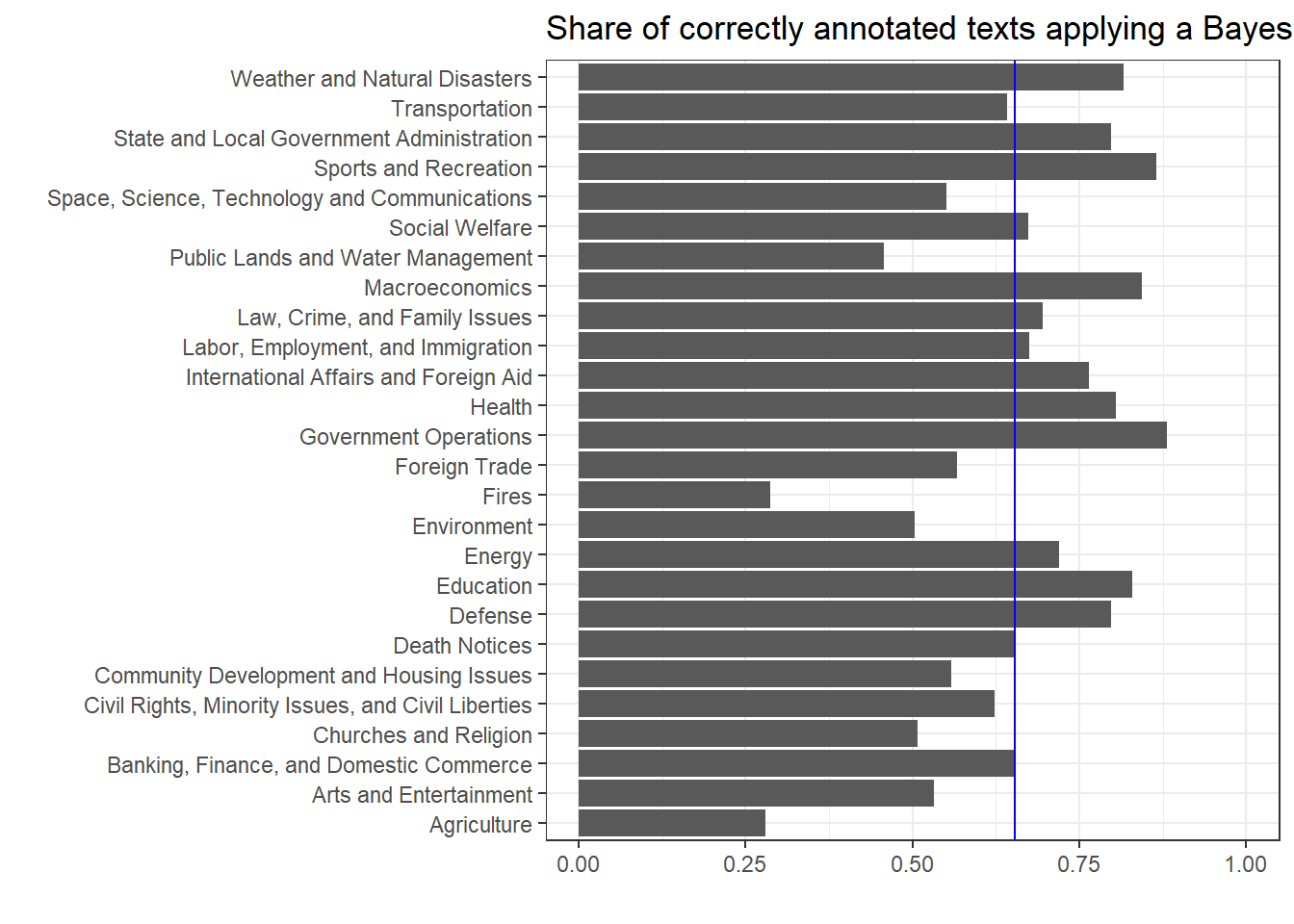
Why does the accuracy of classification by category vary so much? On the one hand, this has to do with the uniqueness of the vocabulary in certain subject areas (e.g., sport and education versus agriculture), but on the other hand it is mainly related to the sample size. The categories fire, agriculture, and public property are simply too small to extract a reliable vocabulary for classification.
Which terms are particularly strongly associated with a particular content-analysis category on the basis of coding? By extracting certain indicators from the model data structure, we can easily answer this question. Below we plot the five most relevant terms for six of the 26 content analysis categories. Within the model, the variable PwGc denotes the empirical probability of the term for the class. The call is a little more complicated because it is implemented with dplyr and ggplot and is not included in quanteda.
nb.terms <- as.data.frame(t(modell.NB$PwGc)) %>%
  rownames_to_column("Wort") %>%
  gather(Category, Probability, -Wort) %>%
  arrange(Category, desc(Probability)) %>%
  left_join(labels.categories, by = "Category") %>%
  mutate(Category = as.numeric(Category)) %>%
  group_by(Category) %>%
  mutate(Rang = row_number()) %>%
  filter(Rang <= 3) %>%
  filter(Category <= 4)
ggplot(nb.terms, aes(reorder(Wort, Rang), Probability)) +
  geom_bar(stat = "identity") +
  theme(axis.text.x = element_text(angle = 45, hjust = 1)) +
  xlab("") + ylab("") +
  facet_grid(. ~ Category)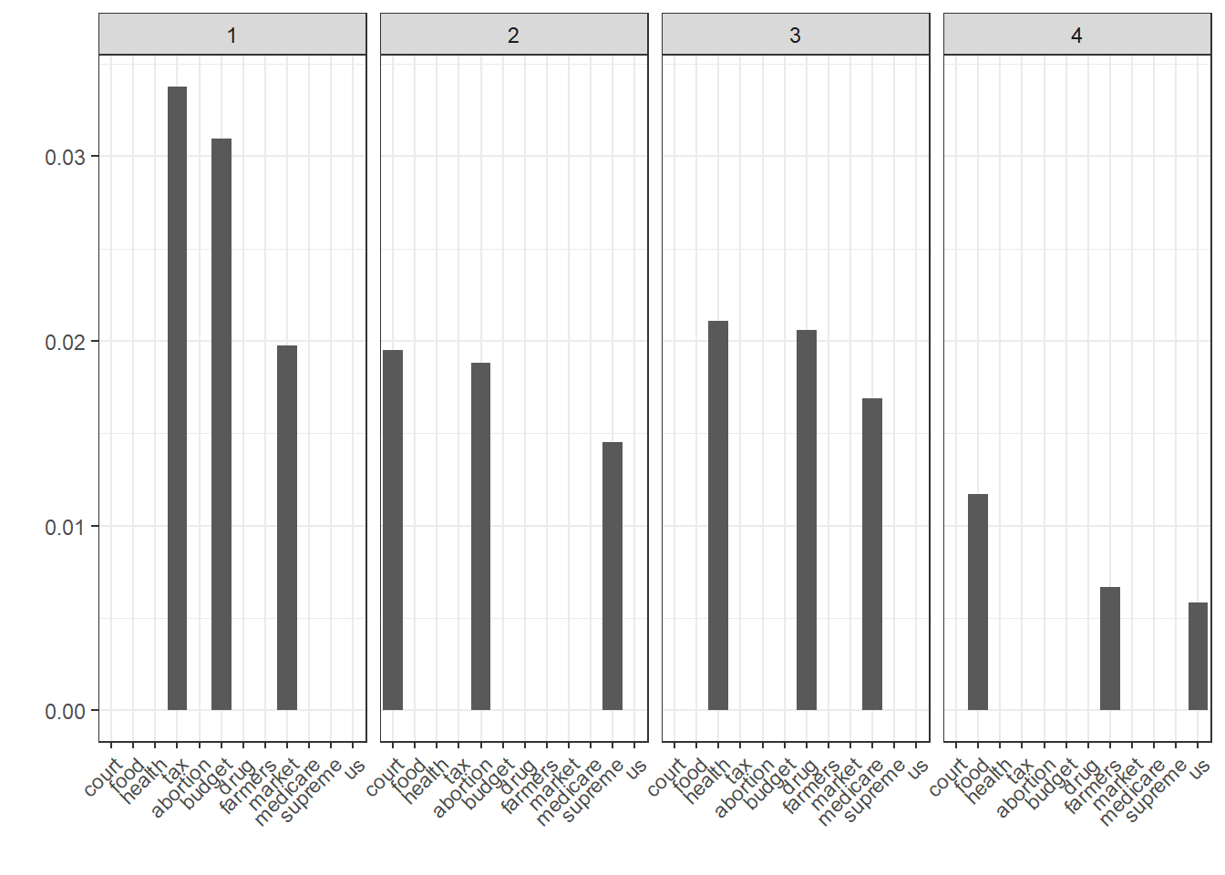
Even if it’s probably obvious: In contrast to the methods used so far, this type of association is based on manual coding (i.e., the decisions made by human coders, and not on the fact that the terms often occur together). Often, however, both are the case at the same time; terms often appear together in contributions that are classified by coders as belonging to the same class.
Things to remember about supervised machine learning
The following characteristics of supervised machine learning are worth bearing in mind:
- quanteda is useful for preparing data that is then subjected to UML/SML/other techniques
- combination with tidyverse leads to more transparent code
- a lot of useful areas I haven’t addressed (scaling models, POS tagging, named entities, word embeddings…)
- validate, validate, validate