Automated Content Analysis with R
Sentiment analysis
Cornelius Puschmann & Mario Haim
Sentiment analysis has its roots in computational linguistics and computer science, but in recent years it has also been increasingly used in the social sciences to automatically classify very different texts, such as parliamentary debates, free text answers in surveys, or social-media discourse. The aim of sentiment analysis is to determine the polarity of a text (i.e., whether the emotions expressed in it are rather positive or negative). This is often done by word lists and by counting terms that were previously assigned to the categories positive or negative.
In many procedures, the result is subsequently scaled through automated classifications. However, such word-list classification may lead to incorrect results, which occur mainly when negation or irony is used, but also when the object of the positive or negative expressions changes or is unclear. Originally, sentiment analysis was tested on product reviews on e-commerce platforms such as Amazon.com, where these issues play a relatively minor role. In the case of press texts or discourse in social media, on the other hand, it is often more difficult to assess what a sentiment rating refers to or what sentiment level should be regarded as ‘normal’. For example, press texts generally express little emotion, and negative terms often predominate, without this necessarily being due to a bad state of the world. Finally, one should bear in mind that sentiment analysis is a heuristic procedure that always produces incorrect individual classifications, which ideally does not carry too much weight when examining some changes in the sentiment course over time.
As far as the technical implementation is concerned, the approach used here is very similar to the application of topical dictionaries insofar as both approaches use very similar procedures. In both cases, a dictionary (‘sentiment/topic dictionary’) is used to group a number of individual terms into one category.
In this chapter we use four sentiment dictionaries in English:
These dictionaries are simply lists of words which are assigned to the categories positive or negative as described above. In some cases there is also a third category neutral. Furthermore, terms could be assigned to more than one category, or besides an assignment of polarity they can also be assigned a sentiment strength. The technique presented here is comparatively primitive because it only counts words, but the procedures can easily be refined (see e.g. this article by Christian Rauh on the validation of political sentiment lexica). Even procedures that use weights or other tricks to reduce the error rate work like this – sentiment analysis is effective, but also anything but witchcraft.
We apply these dictionaries to four data sets: the well-known Sherlock Holmes corpus, a data set from tweets by Donald Trump and Hillary Clinten and a corpus of Swiss daily newspapers with articles on the financial crisis written between 2007 and 2012. We will go into the composition of the corpora later.
Installing/loading R libraries and a corpus
First the necessary libraries are loaded again. New is the library scales which is used for the normalization of sentiment scores. Then, in a second step, the Sherlock corpus is loaded, which we have already saved together with metadata in RData format.
if(!require("quanteda")) {install.packages("quanteda"); library("quanteda")}
if(!require("tidyverse")) {install.packages("tidyverse"); library("tidyverse")}
if(!require("scales")) {install.packages("scales"); library("scales")}
if(!require("lubridate")) {install.packages("lubridate"); library("lubridate")}
load("data/sherlock/sherlock.RData")
theme_set(theme_bw())
Creating an ad-hoc dictionary in quanteda
We begin with a sentiment analysis of the Sherlock Holmes narratives in order to stick to a corpus already familiar from Chapters 1 and 2. In a first step, we create a very simple ad-hoc dictionary of only six terms to illustrate the structure of a dictionary in quanteda. This is done with the quanteda command dictionary(). Dictionary() accepts a number of standard formats (more on this later), but also vectors containing the terms that operationalize an abstract category. Any number of categories can be defined in this way and then ‘filled’ with thousands of terms. Categories with several hierarchical levels are also possible - more about this in the next chapter.
test.lexicon <- dictionary(list(positive.terms = c("happiness", "joy", "light"), negative.terms = c("sadness", "anger", "darkness")))
test.lexicon
## Dictionary object with 2 key entries.
## - [positive.terms]:
## - happiness, joy, light
## - [negative.terms]:
## - sadness, anger, darknessFirst sentiment analysis with Sherlock Holmes corpus
With this dictionary we can do little concrete with our Sherlock Holmes corpus, so we better switch to a real sentiment dictionary. In a second step we thus read the Bing Liu Sentiment Lexicon into R with the command scan. This lexicon contains over 6,700 English terms stored in two simple text files, each containing one word per line. We skip the first 35 lines with the argument skip because they contain meta information about the lexicon. The argument quiet prevents the output of a status message.
positive.words.bl <- scan("dictionaries/bingliu/positive-words.txt", what = "char", sep = "\n", skip = 35, quiet = T)
negative.words.bl <- scan("dictionaries/bingliu/negative-words.txt", what = "char", sep = "\n", skip = 35, quiet = T)
Now we create the dictionary with the help of the text vectors we just read in. This is done again with the function dictionary(), this time with the currently read vectors as argument.
sentiment.dictionary <- dictionary(list(positive = positive.words.bl, negative = negative.words.bl))
str(sentiment.dictionary)
## Formal class 'dictionary2' [package "quanteda"] with 2 slots
## ..@ .Data :List of 2
## .. ..$ :List of 1
## .. .. ..$ : chr [1:2006] "a+" "abound" "abounds" "abundance" ...
## .. ..$ :List of 1
## .. .. ..$ : chr [1:4783] "2-faced" "2-faces" "abnormal" "abolish" ...
## ..@ concatenator: chr " "As you can see, several thousand terms have now been assigned to the two categories of the lexicon. Now we can calculate a DFM, which applies the created lexicon to the corpus.
dfm.sentiment <- dfm(sherlock.corpus, dictionary = sentiment.dictionary)
dfm.sentiment
## Document-feature matrix of: 12 documents, 2 features (0.0% sparse).
## 12 x 2 sparse Matrix of class "dfm"
## features
## docs positive negative
## A Scandal in Bohemia 248 204
## The Red-headed League 272 217
## A Case of Identity 200 194
## The Boscombe Valley Mystery 195 295
## The Five Orange Pips 149 213
## The Man with the Twisted Lip 193 298
## The Adventure of the Blue Carbuncle 200 226
## The Adventure of the Speckled Band 205 375
## The Adventure of the Engineer's Thumb 223 246
## The Adventure of the Noble Bachelor 237 208
## The Adventure of the Beryl Coronet 276 280
## The Adventure of the Copper Beeches 287 311What has happened? All actual mentions of the 6,700 terms contained in the Bing Liu dictionary have been replaced in the twelve Sherlock Holmes novels with their respective categories. All terms that do not appear in the dictionary are simply omitted. This leaves a table with only two columns left - the sum of all positive and negative terms per novel. We will discuss this in detail later, but perhaps you have already noticed that dictionary is used to summarize the columns of a DFM (the words), while the group argument of the dfm() function summarizes the rows (the texts). This dimensional reduction is one of the most useful properties of quanteda.
The following plot shows the sentiment distribution in the twelve Sherlock Holmes stories.
sentiment <- convert(dfm.sentiment, "data.frame") %>%
  gather(positive, negative, key = "Polarity", value = "Words") %>%
  mutate(document = as_factor(document)) %>%
  rename(Novel = document)
ggplot(sentiment, aes(Novel, Words, fill = Polarity, group = Polarity)) + geom_bar(stat='identity', position = position_dodge(), size = 1) + scale_fill_brewer(palette = "Set1") + theme(axis.text.x = element_text(angle = 45, vjust = 1, hjust = 1)) + ggtitle("Sentiment scores in twelve Sherlock Holmes novels") + xlab("")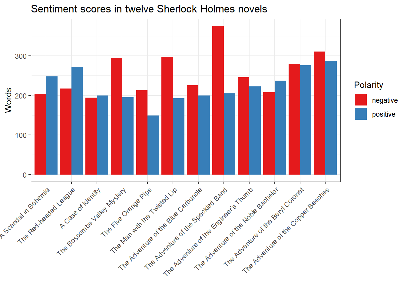
Weighting of sentiment scores
If you remember the problems of absolute word frequencies addressed in the previous chapter, you might prefer to calculate relative frequencies. When using dictionaries, this usually means not only that the appearance of the dictionary terms is measured relative to the total word frequency, but also their proportion relative to each other (i.e., the ratio of positive and negative terms). This has the advantage that one can disregard the large number of all terms that are neither positive nor negative, which makes sense if one is only interested in sentiment only.
The following example illustrates this procedure.
dfm.sentiment.prop <- dfm_weight(dfm.sentiment, scheme = "prop")
dfm.sentiment.prop
## Document-feature matrix of: 12 documents, 2 features (0.0% sparse).
## 12 x 2 sparse Matrix of class "dfm"
## features
## docs positive negative
## A Scandal in Bohemia 0.5486726 0.4513274
## The Red-headed League 0.5562372 0.4437628
## A Case of Identity 0.5076142 0.4923858
## The Boscombe Valley Mystery 0.3979592 0.6020408
## The Five Orange Pips 0.4116022 0.5883978
## The Man with the Twisted Lip 0.3930754 0.6069246
## The Adventure of the Blue Carbuncle 0.4694836 0.5305164
## The Adventure of the Speckled Band 0.3534483 0.6465517
## The Adventure of the Engineer's Thumb 0.4754797 0.5245203
## The Adventure of the Noble Bachelor 0.5325843 0.4674157
## The Adventure of the Beryl Coronet 0.4964029 0.5035971
## The Adventure of the Copper Beeches 0.4799331 0.5200669This DFM is also easy to plot.
sentiment <- convert(dfm.sentiment.prop, "data.frame") %>%
  gather(positive, negative, key = "Polarity", value = "Share") %>%
  mutate(document = as_factor(document)) %>%
  rename(Novel = document)
ggplot(sentiment, aes(Novel, Share, fill = Polarity, group = Polarity)) + geom_bar(stat='identity', position = position_dodge(), size = 1) + scale_fill_brewer(palette = "Set1") + theme(axis.text.x = element_text(angle = 45, vjust = 1, hjust = 1)) + ggtitle("Sentiment scores in twelve Sherlock Holmes novels (relative)")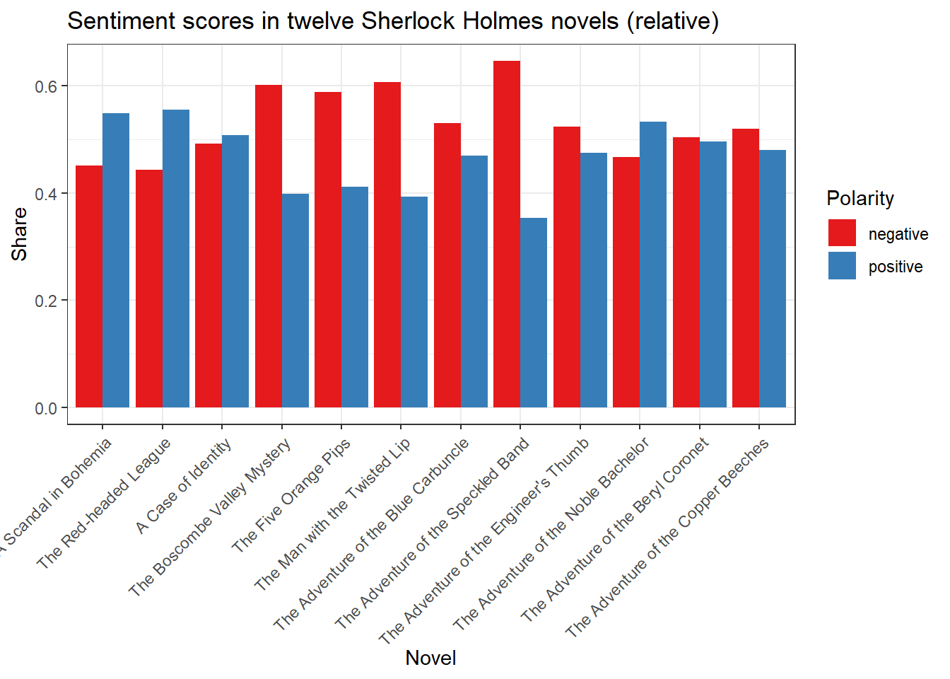
Calculation and scaling of positive and negative sentiment shares
The representation of sentiment shares within the twelve narratives can be further improved by refraining from depicting both polarities. Since in these applications the negative polarity simply results in the inversion of the positive sentiment, this is sufficient. We also rescale the values using rescale so that they are between -1 and +1.
sentiment <- convert(dfm.sentiment.prop, "data.frame") %>%
  rename(Novel = document, Sentiment = positive) %>%
  select(Novel, Sentiment) %>%
  mutate(Sentiment = rescale(Sentiment, to = c(-1,1))) %>%
  mutate(Novel = as_factor(Novel))
ggplot(sentiment, aes(Novel, Sentiment, group = 1)) + geom_line(size = 1) + geom_hline(yintercept = 0, linetype = "dashed", color = "lightgray") + theme(axis.text.x = element_text(angle = 45, vjust = 1, hjust = 1)) + ggtitle("Combined sentiment scores in twelve Sherlock Holmes novels") + xlab("")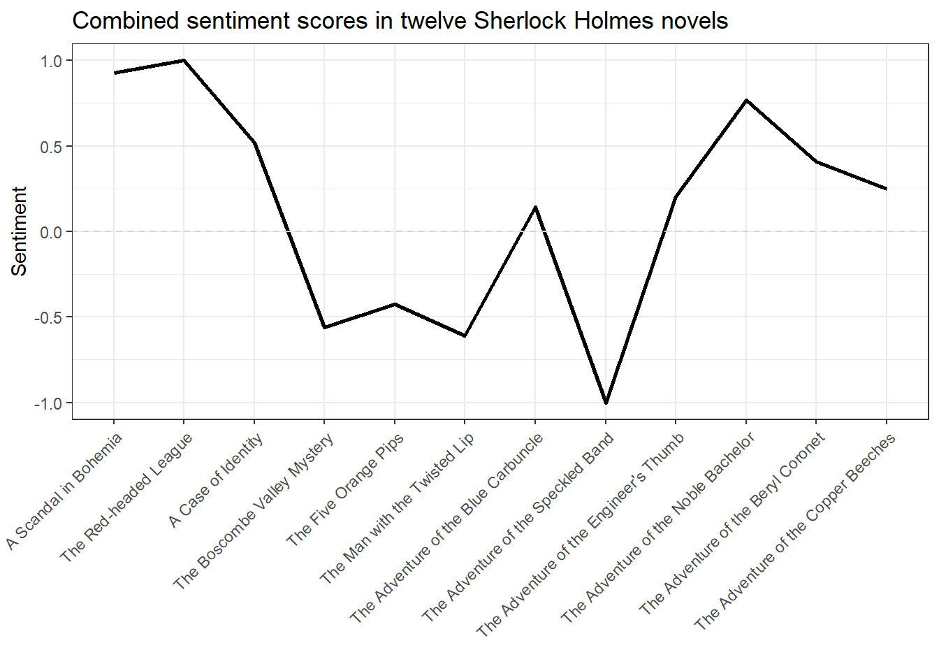
We note: The novels at the beginning of the Sherlock Holmes Cyclus are a bit more positive, while the middle is darker. In the end, however, the mood lifts again – at least in comparison. Contrasting this representation with the first plot, it becomes clear why calculated frequencies are often a good approach. On the other hand, you cannot take for granted that the sentiment in ‘The Adventure of the Speckled Band’ is exclusively negative (i.e., ‘0% positive’), because this is an artefact of our proportional scaling. It is only proportionally more negative than in the other eleven stories.
Sentiment analysis with Twitter data from Donald Trump and Hillary Clinton
Let us now turn to a more recent example, namely the analysis of the sentiment in the tweets of Donald Trump and Hillary Clinton before, during, and after the US presidential campaign of 2016.
First load like the Trump and Clinton Twitter datasets (already combined in a corpus object and saved as RData file). This data was collected from various online archives and through the Twitter API. I am not going to go into the creation of the corpus in more detail here, but this will be explained later.
load("data/twitter/trumpclinton.RData")
trumpclinton.stats.monthly
The table shows the already monthly aggregated tweet numbers. Here are some examples for tweets of the two candidates (again you can scroll to the right/left with the arrow icon):
trumpclinton.sample <- corpus_sample(trumpclinton.corpus, size = 20)
bind_cols(text = texts(trumpclinton.sample), docvars(trumpclinton.sample))
First, let’s plot the words (or more precisely the tokens) per month for Hillary Clinton and Donald Trump from April 2015 to April 2017 to get an impression of their activity. This corresponds relatively well to the number of tweets, since the variation in length is not too strong.
Attention: Here the color indicates the candidate, not the sentiment.
ggplot(trumpclinton.stats.monthly, aes(as.Date(paste(Year, Month, "01", sep = "-")), Tweets, group = Candidate, col = Candidate)) +
  geom_line(size = 1) +
  scale_colour_brewer(palette = "Set1") +
  scale_x_date(date_breaks = "2 months", date_labels = "%b %Y") +
  theme(axis.text.x = element_text(angle = 45, hjust = 1)) +
  ggtitle("Trump vs. Clinton: Tweets per month (2015-2017)") +
  xlab("")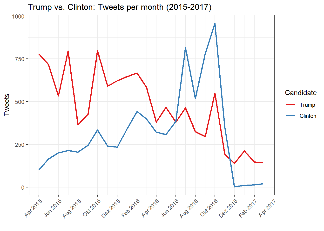
It can be observed that Hillary Clinton became much more active in the six months leading up to the November 2016 election, while Donald Trump, in direct comparison to his continued presence on Twitter since 2009, was rather less active.
We now first create a DFM for each of the candidates and apply the Bing Liu Sentiment Dictionary again. We start with Donald Trump and filter the corpus according to his tweets, which we then aggregate according to month and year using the argument groups (otherwise you get the sentiment result for every single tweet, which is not necessarily interpretable with roughly 20,000 tweets). Then we use convert to create a data frame, which we edit a bit to make it easier to plot.
corpus.trump <- corpus_subset(trumpclinton.corpus, Candidate == "Trump")
dfm.trump <- dfm(corpus.trump, groups = c("Month", "Year"), dictionary = sentiment.dictionary)
sentiment.trump <- convert(dfm.trump, "data.frame") %>%
  gather(positive, negative, key = "Polarity", value = "Words") %>%
  mutate(Date = as.Date(paste("01", document, sep = "."), "%d.%m.%Y")) %>%
  filter(Date >= "2015-04-01" & Date <= "2017-04-01")
ggplot(sentiment.trump, aes(Date, Words, color = Polarity, group = Polarity)) + geom_line(size = 1) + scale_colour_brewer(palette = "Set1") + scale_x_date(date_breaks = "2 months", date_labels = "%b %Y") + ggtitle("Sentiment scores for Donald Trump") + xlab("month") + theme(axis.text.x = element_text(angle = 45, hjust = 1)) + xlab("")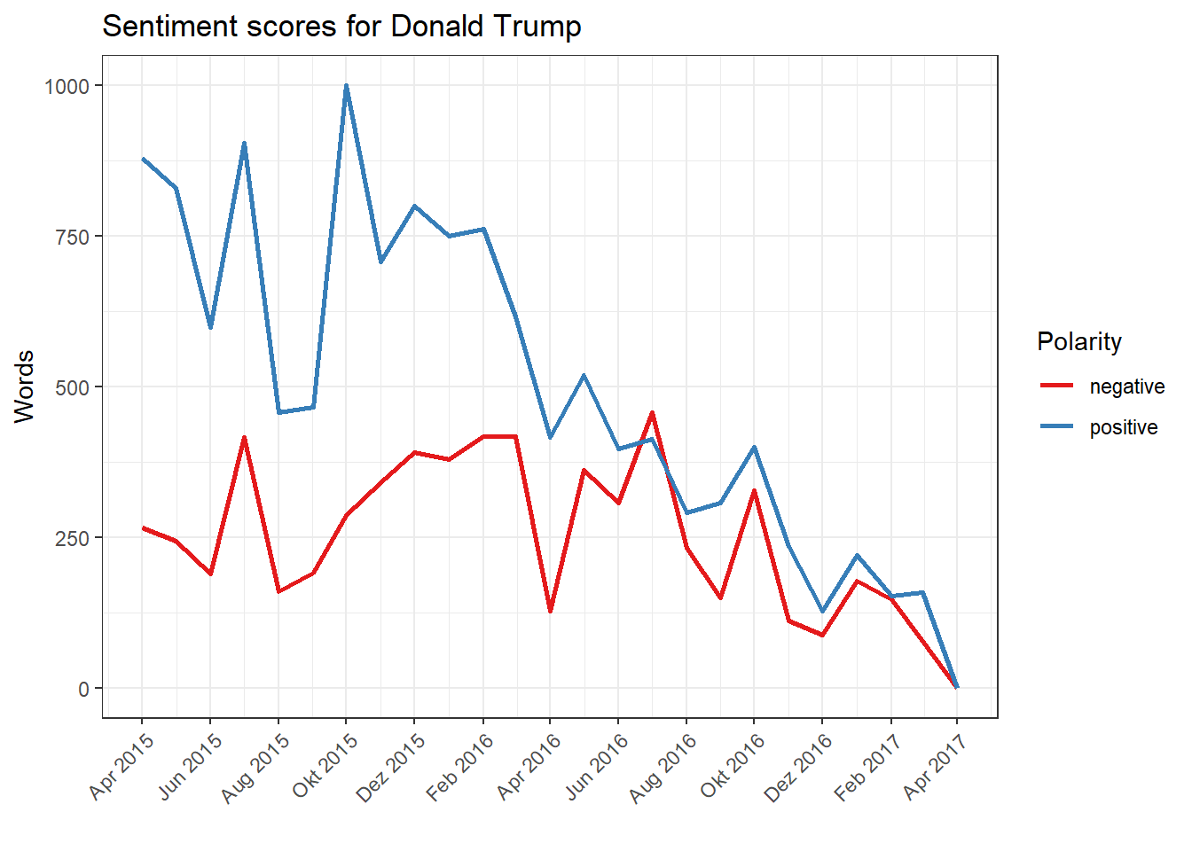
We repeat the exact same process for Hillary Clinton. We filter their tweets out of the whole body, group a DFM by month and year using the dictionary, and then plot the result.
corpus.clinton <- corpus_subset(trumpclinton.corpus, Candidate == "Clinton")
dfm.clinton <- dfm(corpus.clinton, groups = c("Month", "Year"), dictionary = sentiment.dictionary)
sentiment.clinton <- convert(dfm.clinton, "data.frame") %>%
  gather(positive, negative, key = "Polarity", value = "Words") %>%
  mutate(Date = as.Date(paste("01", document, sep = "."), "%d.%m.%Y")) %>%
  filter(Date >= "2015-04-01" & Date <= "2017-04-01")
ggplot(sentiment.clinton, aes(Date, Words, color = Polarity, group = Polarity)) + geom_line(size = 1) + scale_colour_brewer(palette = "Set1") + scale_x_date(date_breaks = "2 months", date_labels = "%b %Y") + ggtitle("Sentiment scores for Hillary Clinton") + xlab("month") + theme(axis.text.x = element_text(angle = 45, hjust = 1)) + xlab("")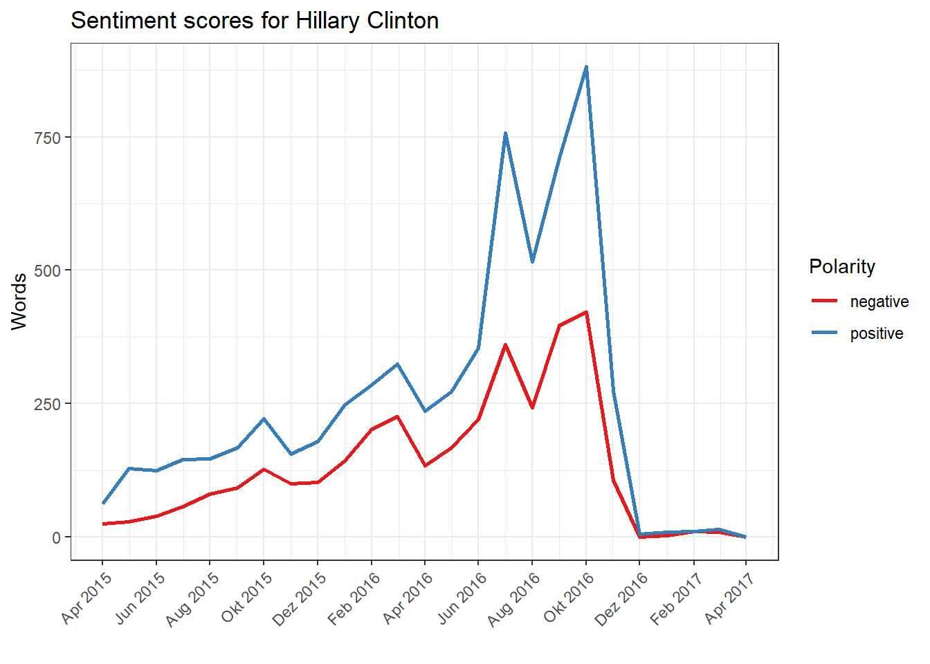
In a direct comparison, both candidates tweet more positively than negatively, which may come as a surprise. However, the overall gap between positive and negative sentiment in Hillary Clinton is high, and particularly pronounced in the hot phase of the election campaign. For Donald Trump, on the other hand, the negative sentiment dominates in July 2016 whereas in February 2017 positive and negative terms are roughly the same. For Trump, strong fluctuations are also noticeable which are missing in Clinton’s tweets.
What does the Twitter activity of both candidates look like in a direct comparison? We skip the second step from the above analysis and proceed immediately to plot only the calculated relative share of the positive sentiment for both polticians. We also limit the time period by cutting right after the election in November 2017. This should eliminate the very low number of tweets by Hillary Clinton after the election which would make comparison more difficult and potentially lead to distortions.
dfm.trump.prop <- dfm_weight(dfm.trump, scheme = "prop")
sentiment.trump.prop <- convert(dfm.trump.prop, "data.frame") %>%
  gather(positive, negative, key = "Polarity", value = "Sentiment") %>%
  mutate(Date = as.Date(paste("01", document, sep = "."), "%d.%m.%Y")) %>%
  filter(Date >= "2015-04-01" & Date <= "2016-11-01") %>%
  mutate(candidate = "Trump")
dfm.clinton.prop <- dfm_weight(dfm.clinton, scheme = "prop")
sentiment.clinton.prop <- convert(dfm.clinton.prop, "data.frame") %>%
  gather(positive, negative, key = "Polarity", value = "Sentiment") %>%
  mutate(Date = as.Date(paste("01", document, sep = "."), "%d.%m.%Y")) %>%
  filter(Date >= "2015-04-01" & Date <= "2016-11-01") %>%
  mutate(candidate = "Clinton")
sentiment.trumpclinton <- bind_rows(sentiment.trump.prop, sentiment.clinton.prop) %>%
  filter(Polarity == "positive") %>%
  mutate(Sentiment = rescale(Sentiment, to = c(-1,1))) %>%
  mutate(Candidate = as_factor(candidate)) %>%
  select(Date, Sentiment, Candidate)
ggplot(sentiment.trumpclinton, aes(Date, Sentiment, colour = Candidate, group = Candidate)) +
  geom_line(size = 1) +
  geom_hline(yintercept = 0, linetype = "dashed", color = "lightgray") +
  scale_colour_brewer(palette = "Set1") +
  scale_x_date(date_breaks = "1 month", date_labels = "%b %Y") +
  theme(axis.text.x = element_text(angle = 45, hjust = 1)) +
  ggtitle("Calculated sentiment scores for both candidates") +
  xlab("")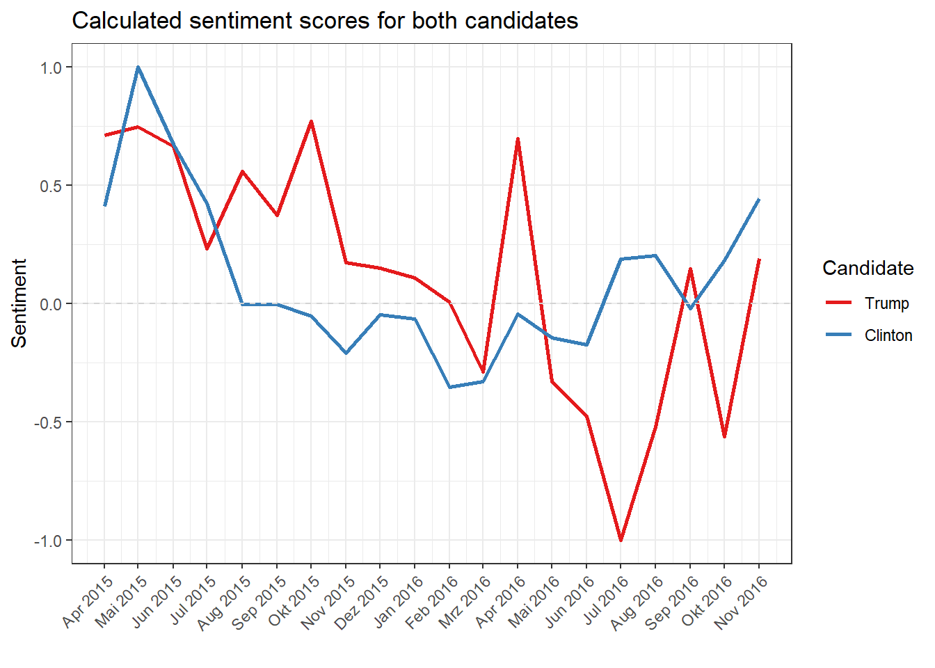
The normalization shows the highs and lows, relative to the sentiment course in the total time, and calculates the positive and negative terms as before. In July 2016, Trump tweets strongly negative, but this does not mean that the proportion of negative terms was generally much higher than the proportion of positive terms. Interesting references can be made to the context of the US elections, including the nomination of Donald Trump and Hillary Clinton as Republican and Democrat candidates, respectively, and the revelation of [hacked emails from the DNC] (https://en.wikipedia.org/wiki/2016_Democratic_National_Committee_email_leak), which already in 2016 brought up the accusation of a targeted manipulation attempt by Russia. Numerous tweets by Trump criticize the media for this what Trump considered to be false allegations. The reason for Trump’s nevertheless partly high sentiment values lies in the use of many positive adjectives and superlatives (‘great’, ‘best’), which occur naturally in sentiment dictionaries.
By the way: The code for this analysis can be simplified to the extent that a number of steps are necessary only for the creation of the plot, but not for the creation of the weighted DFM and the use of the dictionary.
Comparison of AFINN, Bing Liu and NRC sentiment dictionaries
What are the differences between different dictionaries? Since different dictionaries also contain different terms, this question is quite significant. To answer them, we calculate three different DFMs using Donald Trump’s Tweets, each with a different lexicon. First of all, we read in all three dictionaries, namely AFINN, Bing Liu and NRC.
sentiment.dictionary.bingliu <- dictionary(list(positive = scan("dictionaries/bingliu/positive-words.txt", what = "char", sep = "\n", skip = 35, quiet = T), negative = scan("dictionaries/bingliu/negative-words.txt", what = "char", sep = "\n", skip = 35, quiet = T)))
sentiment.dictionary.nrc <- dictionary(list(positive = scan("dictionaries/nrc/pos.txt", what = "char", sep = "\n", quiet = T), negative = scan("dictionaries/nrc/neg.txt", what = "char", sep = "\n", quiet = T)))
afinn <- read.csv("dictionaries/AFINN-111.txt", header = F, sep = "\t", stringsAsFactors = F)
sentiment.dictionary.afinn <- dictionary(list(positive = afinn$V1[afinn$V2>0], negative = afinn$V1[afinn$V2<0]))
While the import for the Bing Liu lexicon and the NRC Emotions lexicon is very easy, the AFINN dictionary has a special format where a number between -5 and +5 describes the polarity from very negative to very positive. We do not use this special advantage here, but treat all terms as ‘simply’ negative (< 0) or positive (> 0).
Again, the dictionary is used, grouped by month and year, and then proportionally weighted – for each of the three dictionaries.
dfm.trump.bingliu <- dfm_weight(dfm(corpus.trump, groups = c("Month", "Year"), dictionary = sentiment.dictionary.bingliu))
dfm.trump.nrc <- dfm_weight(dfm(corpus.trump, groups = c("Month", "Year"), dictionary = sentiment.dictionary.nrc))
dfm.trump.afinn <- dfm_weight(dfm(corpus.trump, groups = c("Month", "Year"), dictionary = sentiment.dictionary.afinn))
The three DFMs are then converted into data frames and a variable is added to identify the lexicon.
sentiment.trump.bingliu <- convert(dfm.trump.bingliu, "data.frame") %>% mutate(Dictionary = "Bing Liu")
sentiment.trump.nrc <- convert(dfm.trump.nrc, "data.frame") %>% mutate(Dictionary = "NRC")
sentiment.trump.afinn <- convert(dfm.trump.afinn, "data.frame") %>% mutate(Dictionary = "AFINN")
Finally, a common data frame is put together and transformed. The resulting plot shows the calculated sentiment scores of Donald Trump for all three dictionaries.
sentiment.trump.combined <- bind_rows(sentiment.trump.bingliu, sentiment.trump.nrc, sentiment.trump.afinn) %>%
  gather(positive, negative, key = "Polarity", value = "Sentiment") %>%
  filter(Polarity == "positive") %>%
  mutate(Date = as.Date(paste("01", document, sep = "."), "%d.%m.%Y")) %>%
  filter(Date >= "2015-04-01" & Date <= "2017-03-01") %>%
  mutate(Sentiment = rescale(Sentiment, to = c(-1,1))) %>%
  select(Date, Dictionary, Sentiment)
ggplot(sentiment.trump.combined, aes(Date, Sentiment, colour = Dictionary, group = Dictionary)) + geom_line(size = 1) + scale_colour_brewer(palette = "Dark2") + geom_hline(yintercept = 0, linetype = "dashed", color = "lightgray") + scale_x_date(date_breaks = "2 months", date_labels = "%b %Y") + ggtitle("Combined sentiment scores for Donald Trump with three dictionaries") + xlab("") + theme(axis.text.x = element_text(angle = 45, hjust = 1))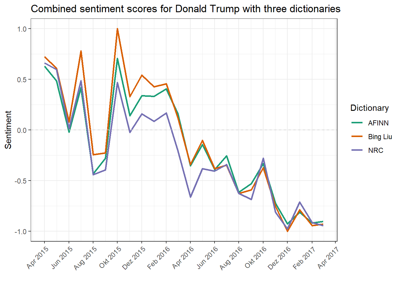
As we can see, the trend of the three dictionaries is clearly the same, but there are striking differences. AFINN and Bing Liu are slightly more positive about NRC. To some extent, the intensity of the deflections also differs in both polarity directions. One reason for the variation is the length of the word lists, since more extensive lists provide better coverage of the terms actually used. In principle, the three dictionaries do not differ significantly and, for example, clearly agree in their measurement of the sentiment fluctuation between September and November 2016.
Sentiment in two subreddits using the Lexicoder Sentiment Dictionary (LSD2015)
Next, we turn to an example that comes from Reddit, rather than Twitter. As before, we begin by loading and inspecting the data.
load("data/reddit.RData")
as.data.frame(reddit.stats)
The corpus contains approximately 20,000 comments posted to two subreddits, ‘science’ and ‘syriancivilwar’. We proceed to calculate sentiment scores for these messages using the Lexicoder Sentiment Dictionary (LSD2015), which was automatically loaded with quanteda. We apply log. average weighting and truncate the result, thus determining a polarity score per comment rather than per word (note that there are different strategies for doing this).
reddit.dfm <- dfm(reddit.corpus, dictionary = data_dictionary_LSD2015) %>%
  dfm_remove(c("neg_positive", "neg_negative"))
reddit.sentiment <- dfm_weight(reddit.dfm, scheme = "logave") %>%
  convert("data.frame") %>%
  mutate(positive = trunc(positive), negative = trunc(negative)) %>%
  mutate(neutral = positive == negative) %>%
  left_join(reddit.stats, by = c("document" = "Text"))
## Warning: Column `document`/`Text` joining character vector and factor,
## coercing into character vectorsentiment <- ""
sentiment[reddit.sentiment$positive==1] <- "positive"
sentiment[reddit.sentiment$negative==1] <- "negative"
sentiment[reddit.sentiment$neutral==T] <- "neutral"
reddit.sentiment.share <- reddit.sentiment %>%
select(document, structure, comm_date, subreddit, user) %>%
data.frame(Sentiment = sentiment)
reddit.sentiment.shareNext, we plot aggregate results per subreddit.
reddit.sentiment.share <- data.frame(table(reddit.sentiment.share$Sentiment, reddit.sentiment.share$subreddit))
colnames(reddit.sentiment.share) <- c("Sentiment", "Subreddit", "Share")
ggplot(reddit.sentiment.share, aes(Subreddit, Share, colour = Sentiment, fill = Sentiment)) + geom_bar(stat="identity") + scale_colour_brewer(palette = "Set1") + scale_fill_brewer(palette = "Pastel1") + ggtitle("Sentiment shares in two subreddits") + xlab("") + ylab("Comments")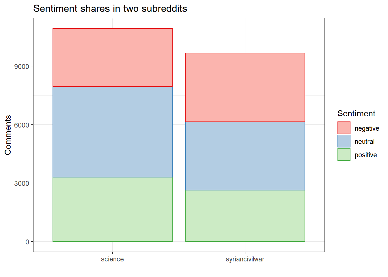
Some example posts (shown here, rather than the comments that we have used for the sentiment analysis) can be used to illustrate which threads contain comments with particular polarity in them.
data.frame(reddit.sentiment, sentiment) %>% filter(sentiment == "positive") %>% sample_n(10) %>% select(sentiment, subreddit, title)data.frame(reddit.sentiment, sentiment) %>% filter(sentiment == "negative") %>% sample_n(10) %>% select(sentiment, subreddit, title)data.frame(reddit.sentiment, sentiment) %>% filter(sentiment == "neutral") %>% sample_n(10) %>% select(sentiment, subreddit, title)Things to remember about sentiment and dictionary analysis
The following characteristics of dictionary-based approaches are worth bearing in mind:
- dictionaries are excellent at reducing complexty (many words -> few(er) categories)
- this works most reliably when the terms comprising the dictionary are informative and domain-speficic (think policy areas, science, business…)
- widely used dictionaries such as LIWC can be assumed to have a certain level of validity that an ad-hoc dictionary may not have
- however, custom-built dictionaries may fit your data better
- a limitation of dictionaries is that they assign words to exclusive categories – more sophisticated approaches can overcome this constraint