Automated Content Analysis with R
Word and text metrics
Cornelius Puschmann & Mario Haim
This second chapter focuses on the analysis of words and texts. At first glance, the metrics presented here may not immediately seem particularly relevant to social-science issues. This is partly due to the fact that we are not yet dealing here with abstract concepts such as sentiment or topic, which will be the focus in the following chapters. However, with aspects such as term frequency and the similarity of texts, which may appear to be closer to linguistics, we look at equally important concepts as they form the basis of the higher-level procedures and can also be used to work on interesting social-science questions.
Some examples: * Which terms are particularly distinctive for a political movement or party? * How linguistically complex are news items in different media (tabloid vs. broadsheet)? * What other words are linked to a key social term (‘climate’, ‘migration’, ‘justice’, ‘digitisation’) and how do they change over time? * How similar are online comments on different topics?
These and similar questions will be addressed in the following sections – but first we will introduce the functions that allow you to work with words and texts in quanteda.
Installing/loading R libraries
First, the necessary libraries are loaded again.
if(!require("quanteda")) {install.packages("quanteda"); library("quanteda")}
if(!require("tidyverse")) {install.packages("tidyverse"); library("tidyverse")}
theme_set(theme_bw())
Second, the Sherlock corpus is loaded, which we already created in the first chapter using readtext() from the raw text. However, this time, we will load the RData file, which is the already prepared corpus. In addition, the RData file also contains a data frame created with summary() with the corpus metadata. On the one hand, this saves us having to create a corpus; on the other hand, the RData format is compressed and thus cuts on hard-drive ressources, which is quite noticeable with text data.
Next, we calculate a DFM based on the corpus object (see Chapter 1), because we need it later.
load("data/sherlock/sherlock.RData")
sherlock.dfm <- dfm(sherlock.corpus, remove_numbers = TRUE, remove_punct = TRUE, remove_symbols = TRUE, remove = stopwords("english"))
sherlock.dfm
## Document-feature matrix of: 12 documents, 8,489 features (79.1% sparse).Creating concordances
One of the simplest functions of quanteda is the possibility of concordances (also called KWIC), which is the extraction of a search term and its surrounding sentence context from a corpus. Concordances can be created in quanteda for single words, but also for phrases. Oftentime, exporting a concordance (e.g., as a CSV file which can be opened with Excel) is particularly useful besides the representation within R. This can be done with the function write_delim().
*Note: The concordance table may be scrolled with the small arrow at the top right.
concordance <- kwic(sherlock.corpus, "data")
concordance
concordance <- kwic(sherlock.corpus, phrase("John|Mary [A-Z]+"), valuetype = "regex", case_insensitive = FALSE)
concordanceconcordance <- kwic(sherlock.corpus, c("log*", "emot*"), window = 10, case_insensitive = FALSE)
concordancewrite_delim(concordance, path = "concordance.csv", delim = ";") # file is Excel compatibleThe concordances consist of the metadata (text name and position), the left context, the search term itself, and the right context. The first concordance contains all occurrences of the term ‘data’, the second contains all occurrences of the names ‘John’ and ‘Mary’ followed by another word in upper case (usually the surname). The third concordance finally contains the word fragments ‘log’ and ‘emot’, words like ‘logical’ and ‘emotional’, but also the plural form ‘emotions’. Strictly speaking, these are not word stems, because the inflection form of irregular words deviates completely from the lemma (see ‘go’ and ‘went’). However, in most social-science application scenarios it is already sufficient to identify different word variants by using placeholders (*). Here, quanteda provides a number of useful features which are described in detail in the documentation of kwic().
Next, we calculate the frequency and dispersion of tokens per narrative, which contain the terms ‘dark’ and ‘light’.
term1 <- kwic(sherlock.corpus, "dark", valuetype = "regex", case_insensitive = FALSE) %>% group_by(docname) %>% summarise(hits = n()) %>% mutate(percentage = hits/(sherlock.stats$Tokens/100), searchterm = "dark") %>% arrange(desc(percentage))
term2 <- kwic(sherlock.corpus, "light", valuetype = "regex", case_insensitive = FALSE) %>% group_by(docname) %>% summarise(hits = n()) %>% mutate(percentage = hits/(sherlock.stats$Tokens/100), searchterm = "light") %>% arrange(desc(percentage))
term1term2Again we first use the function kwic(), but here in combination with several functions from the package dplyr (tidyverse). These functions have nothing to do with quanteda, but are useful for converting any data to R (if you want to know more, have a look at this book). While previously the resulting concordance was simply output, the result is now processed using the functions group_by(), summary(), mutate(), and arrange(). We take advantage of the fact that in a KWIC result all information is already available to calculate the absolute and relative frequency of a term (here ‘light’ and ‘dark’) in a series of documents. We have simply derived the percentage by means of the rule of three (with hits/(sherlock.stats$Tokens/100)).
Word frequencies, however, can be implemented much more easily with quanteda’s own function textstat_frequency(), which we will use consistently from now on. We now plot both the absolute and relative frequencies of the two terms.
terms.combined <- bind_rows(term1, term2)
terms.combined$docname <- factor(terms.combined$docname, levels = levels(sherlock.stats$Text))
ggplot(terms.combined, aes(docname, hits, group = searchterm, fill = searchterm)) +
  geom_bar(stat='identity', position = position_dodge(), size = 1) +
  scale_fill_brewer(palette = "Set1") +
  theme(axis.text.x = element_text(angle = 45, vjust = 1, hjust = 1)) +
  ggtitle("Frequency of search terms \"dark\" and \"light\" per novel (absolute)") +
  xlab("") + ylab("words (total)")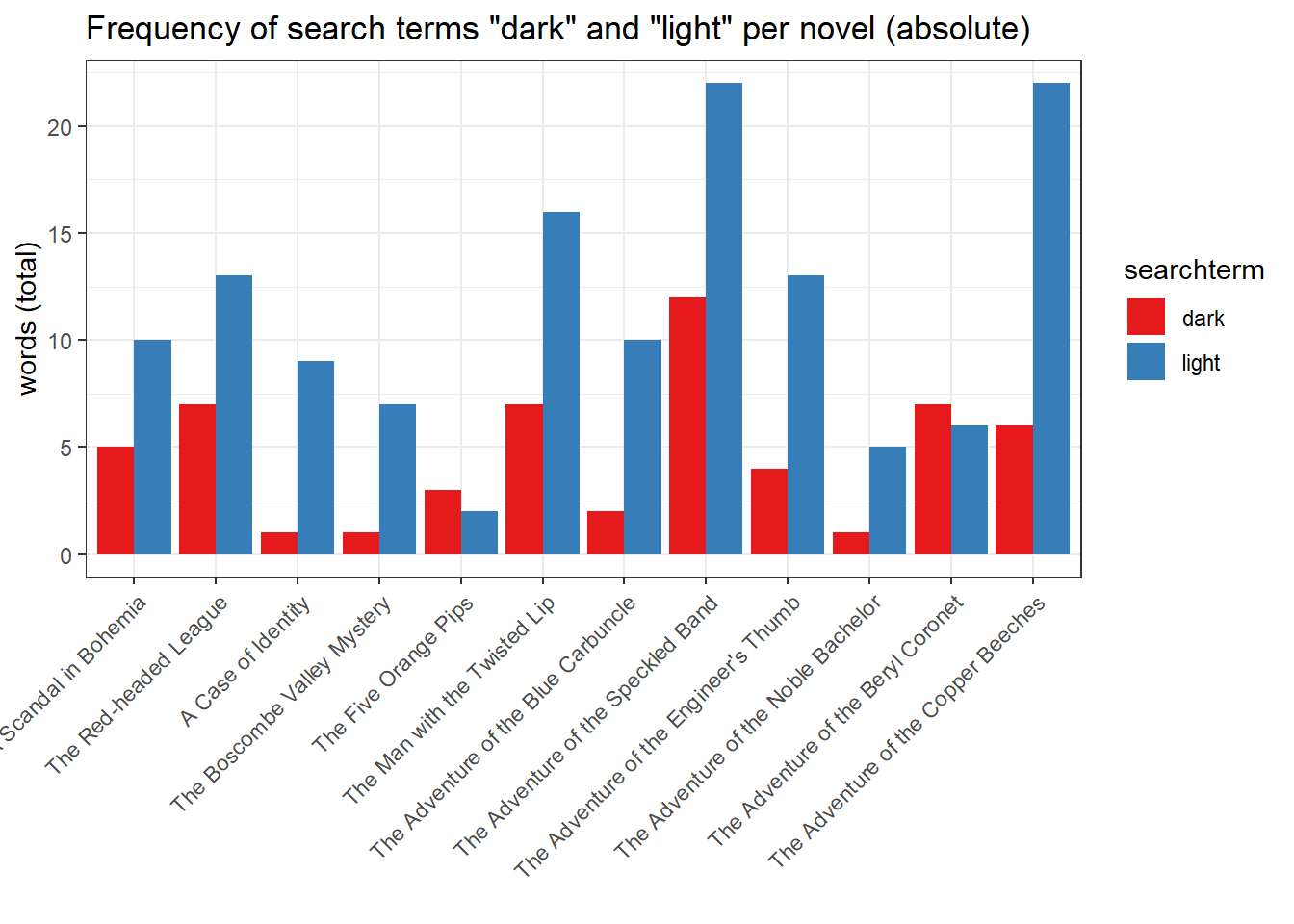
ggplot(terms.combined, aes(docname, percentage, group = searchterm, fill = searchterm)) +
  geom_bar(stat='identity', position = position_dodge(), size = 1) +
  scale_fill_brewer(palette = "Set1") +
  theme(axis.text.x = element_text(angle = 45, vjust = 1, hjust = 1)) +
  ggtitle("Frequency of search terms \"dark\" and \"light\" per novel (relative)") +
  xlab("") + ylab("words (%)")
The first plot shows the absolute frequency of the two terms, while the second plot shows the relative percentage of the term in the total number of words of the respective novel. Why are the two plots almost identical? This has to do with the relatively similar word count of the novels (between 8,500 and 12,000 tokens). If two corpora are of very different size, a normalization of the word frequencies is extremely important, since otherwise the results are significantly distorted. Even so, there are differences when you compare the share of ‘The Adventure of the Speckled Band’ and ‘The Adventure of the Copper Beeches’. While the number of absolute hits on ‘light’ is identical in both novels, the relative proportion on ‘Speckled Band’ drops in comparison.
What to do if you are less interested in the frequency than in the position of the search terms? Plotting the term dispersion as ‘xray-plot’ can be useful, for which the function textplot_xray exists. The X-axis represents the position within the text at which the search term occurs.
textplot_xray(kwic(sherlock.corpus, "dark", valuetype = "regex", case_insensitive = FALSE)) + ggtitle("Lexical dispersion of \"happy\" in Sherlock Holmes")
textplot_xray(kwic(sherlock.corpus, "light", valuetype = "regex", case_insensitive = FALSE)) + ggtitle("Lexical dispersion of \"light\" in Sherlock Holmes")
Collocations
We will now move on to the so-called text statistics. These are functions that can be used to analyze words and texts with a view to their similarity to or distance from other words or texts. An important function in this context is the extraction of collocations. The collocates of a term are terms that often occur together. The process is inductive.
Below we use the function textstat_collocations(), which detects frequent collocates in the Sherlock Holmes corpus. Using write_delim, the result is then saved as an Excel-compatible CSV file.
sherlock.tokens <- tokens(sherlock.corpus)
collocations <- textstat_collocations(sherlock.tokens, min_count = 10)
arrange(collocations, desc(count))
arrange(collocations, desc(lambda))write_delim(collocations, path = "collocations.csv", delim = ";") # file is Excel compatibleIn the two tables, collocation shows us the collocate and count it’s absolute frequency. The association strength of the collocation is measured with lambda and z (more precisely, z is just a z-standardized lambda. Lambda describes the probability that exactly these two terms follow each other, which has to be differentiated from the absolute frequency, as it does not consider the occurrence of a partial term with all other words in the corpus.
The two tables illustrate this difference. The first table is sorted by absolute frequency, so that common collocates like ‘of the’ or ‘it is’ are at the top. The second table is sorted in descending order by lambda, so that a number of proper names like ‘hosmer angel’ or ‘briony lodge’ lead the list. From a practical point of view, it usually makes more sense to consider proper names as phrases than as individual terms whose common appearance really reveals something about the text. Real collocates, on the other hand, are ‘no doubt’ or ‘young lady’.
Word and text similarity and distance
As already indicated in the first chapter, numerous metrics can be calculated on the basis of a DFM, which reflect the proximity and distance of words and documents to each other. This is done with textstat_simil(). First, we construct a DFM in which each sentence corresponds to a document. This is necessary because word similarities cannot be calculated very reliably with a small number of documents, since similarity is operationalized as co-occurrence within the same document. Then we calculate the word similarity to the term ‘love’ using cosine distance. Other available metrics are ‘correlation’, ‘jaccard’, ‘eJaccard’, ‘dice’, ‘eDice’, ‘simple matching’, ‘hamann’ and ‘faith’, which operationalize word similarity differently.
corpus.sentences <- corpus_reshape(sherlock.corpus, to = "sentences")
dfm.sentences <- dfm(corpus.sentences, remove_numbers = TRUE, remove_punct = TRUE, remove_symbols = TRUE, remove = stopwords("english"))
dfm.sentences <- dfm_trim(dfm.sentences, min_docfreq = 5)
similarity.words <- textstat_simil(dfm.sentences, dfm.sentences[,"good"], margin = "features", method = "cosine")
head(similarity.words[order(similarity.words[,1], decreasing = T),], 10)
## good deal heavens enough pay sense
## 1.00000000 0.19605723 0.17937400 0.11864475 0.09802862 0.09491580
## geese christmas chronicle metallic
## 0.09208185 0.09004503 0.08489527 0.08489527The calculation of word distances with the function textstat_dist() works in similar fashion. Again, we have a large number of distance measures to choose from (‘euclidean’, ‘chisquared’, ‘chisquared2’, ‘hamming’, ‘kullback’). manhattan’, ‘maximum’, ‘canberra’, ‘minkowski’).
distance.words <- textstat_dist(dfm.sentences, dfm.sentences[,"love"], margin = "features", method = "euclidean")
head(distance.words[order(distance.words[,1], decreasing = T),], 10)
## upon said holmes one man mr little now
## 23.60085 22.60531 21.47091 20.97618 18.22087 17.63519 17.34935 16.12452
## see may
## 15.71623 15.19868What does the result suggest? Especially that (not surprisingly) words like ‘upon’ and ‘said’ are very far away from ‘love’ – but not in the sense that they would represent the logical opposite of ‘love’ (in linguistics one speaks of antonymy). This is due to the fact that these terms are almost equally distributed in the corpus (i.e., occur everywhere). With the method of word vectors (which we will not discuss here) and very large data sets, however, such and other semantic relationships can also be identified. The filtering we’ve done at DFM before, excludes terms that might never occur together with ‘love’, and thus would be even more distant, but there are a lot of them. In summary, it can be said that text-statistical proximity and distance measures always require a sufficient amount of data in order to deliver a reliable result, and that the search term itself must occur sufficiently often.
If you look at the documentation of textstat_simil() and textstat_dist(), you will notice that there is a somewhat cryptic hint to the argument ‘margin’. This has two possible settings: ‘documents’ or ‘features’. If you set the parameter to ‘documents’, the metrics discussed are not applied to words but to texts. Below we plot the proximity of the text via cosine similarity (here starting from the first novel, ‘A Case of Identity’).
similarity.texts <- data.frame(Text = factor(sherlock.stats$Text, levels = rev(sherlock.stats$Text)), as.matrix(textstat_simil(sherlock.dfm, sherlock.dfm["A Case of Identity"], margin = "documents", method = "cosine")))
ggplot(similarity.texts, aes(A.Case.of.Identity, Text)) + geom_point(size = 2.5) + ggtitle("Cosine similarity of novels (here for 'A Case of Identity')") + xlab("cosine similarity") + ylab("")
As we can see, the similarity between the novels ‘The Red-headed League’ and ‘The Adventure of the Copper Beeches’ with ‘A Case of Identity’ is somewhat greater than for the other novels.
Keyness
The so-called keyness metric is a convenient measure of the distinctiveness of a term for a certain text (i.e., how strongly the term characterizes the respective text in comparison to the entire corpus). While we have previously examined the distance of words and texts from each other, Keyness takes advantage of the frequency with which words are distributed over texts without taking their position into account. Keyness therefore also works well with longer texts, as long as they differ sufficiently. We calculate the keyness for four texts with textstat_keyness() and plot these keyness statistics for four stories with textplot_keyness().
keyness <- textstat_keyness(sherlock.dfm, target = "A Scandal in Bohemia", measure = "lr")
textplot_keyness(keyness)
keyness <- textstat_keyness(sherlock.dfm, target = "A Case of Identity", measure = "lr")
textplot_keyness(keyness)
keyness <- textstat_keyness(sherlock.dfm, target = "The Five Orange Pips", measure = "lr")
textplot_keyness(keyness)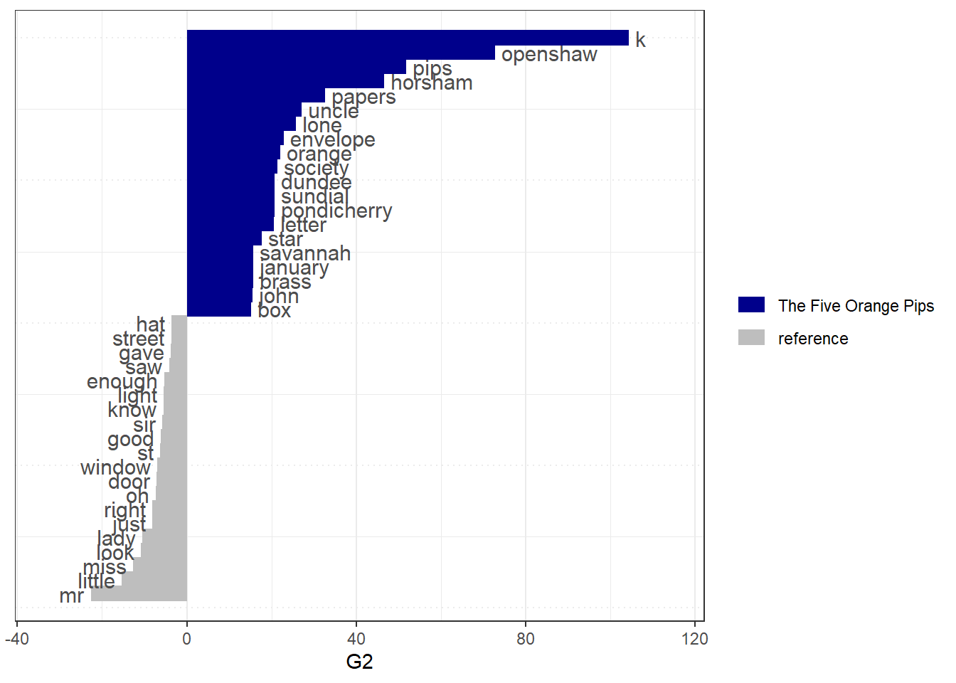
keyness <- textstat_keyness(sherlock.dfm, target = "The Adventure of the Noble Bachelor", measure = "lr")
textplot_keyness(keyness)
If you take a closer look at the four sample texts, it quickly becomes clear that the terms with a high Keyness-value are indeed very distinctive for the respective text, so terms like ‘majesty’ and ‘photograph’ actually only play a role in ‘A Scandal in Bohemia’. Few distinctive terms, on the other hand, are those that appear in other texts but not in the target text. This function is particularly useful if you group texts according to a criterion such as medium, speaker, party, time or manually assigned content category.
Lexical diversity
Measures of lexical diversity are metrics that reflect the diversity of a text with regard to the use of words. An example is the type-token relation already calculated in chapter 1. This describes the word diversity and thus also provides information about the complexity of a text. We calculate numerous metrics for the lexical diversity of the twelve novels with the function textstat_lexdiv().
lexical.diversity <- textstat_lexdiv(sherlock.dfm, measure = "all")
lexical.diversity
write_delim(lexical.diversity, path = "lexicaldiversity.csv", delim = ";") # File is Excel compatibleA superficial comparison of the metrics shows that the texts do not differ very much in their lexical diversity, regardless of which metric is used. This is not necessarily surprising, since they are texts of the same genre and author. Such metrics become more interesting when we want to compare very different genres or authors, such as the programs of parties, texts from different media, or tweets from different users.
Readability indices
Another class of text metrics that can be calculated for a document based on its word composition are so-called readability indices. These are metrics that use text properties to calculate a numerical value that reflects the reading difficulty of a document as accurately as possible. Such indices are used, for example, in the field of education when it comes to determining the level of difficulty of a text for pupils, but also in public administration when it comes to using language that is as clear and accessible as possible, e.g. on a relevant website.
The calculation of numerous readability indices is done in quanteda with textstat_readability(). The result is also stored in an Excel-compatible CSV file.
readability <- textstat_readability(sherlock.corpus, measure = "all")
readability
write_delim(readability, path = "readability.csv", delim = ";") # file is Excel compatibleA nice example of the use of such metrics can be found in the documentation of the textstat_readability() function. While George Washington’s inaugural speech in 1789 still had a Flesh Kincaid Index of 28, the value of Donald Trump’s inaugural speech in 2017 was only 9 (which, however, corresponds to the general trend for inaugural speeches since the middle of the 20th century).
Things to remember about word and text statistics
The following characteristics of word and text statistics are worth bearing in mind:
- concordances are not really a word metric, but can be useful to assess material
- there exists a big toolbox of similary and distance measures to examine both words and texts
- collocations and keyness are convient measures for finding words that are similar (to other words) and that are distinct (for certain texts, relative to all other texts)
- lexical diversity and readibility can act as proxies for textual complexity